Differential equations, a tourist's guide | DE1

Summary

This script delves into the world of differential equations, highlighting their prevalence in describing change in physics and beyond. It introduces ordinary and partial differential equations, using examples like planetary motion and pendulum swings to illustrate their applications. The video aims to provide a conceptual understanding, exploring numerical methods for solving these equations when exact solutions are elusive. It also touches on the challenges of prediction due to chaos theory, emphasizing the beauty and complexity of the mathematical models that underpin our understanding of the universe.

Takeaways

• 📚 Differential equations are fundamental in expressing the laws of physics and are also applicable across various disciplines.
• 🌐 The language of differential equations allows for a deeper understanding of changes in systems, rather than just their absolute states.
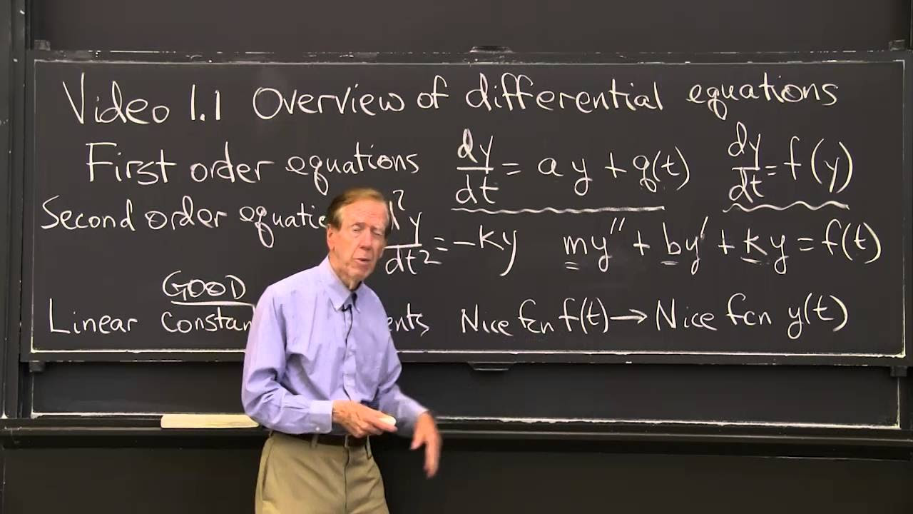
• 🔍 Differential equations are categorized into ordinary differential equations (ODEs), which involve a single variable, and partial differential equations (PDEs), which involve multiple variables.
• 📉 ODEs are used to model systems where a finite set of values change over time, often represented by time itself.
• 🌡 PDEs are employed to describe systems with a continuum of values that evolve over time, such as temperature distribution across a material or fluid velocities.
• 🧮 The study of differential equations often requires knowledge of calculus and, in some cases, basic linear algebra.
• 🌟 Newtonian mechanics uses second-order differential equations to describe motion through the lens of forces leading to acceleration.
• 🔄 The interplay between position and velocity in physics, exemplified by planetary motion, illustrates the complexity of differential equations where acceleration is a function of position.
• 📈 Solving differential equations involves finding functions that describe rates of change, such as velocity and acceleration, based on given conditions.
• 🔍 The concept of phase space, a multi-dimensional representation of all possible states of a system, is crucial for understanding the dynamics of complex systems like the three-body problem.
• 💻 Numerical methods and simulations are essential tools for approximating solutions to differential equations when exact solutions are not feasible, highlighting the practical approach to studying these systems.

Q & A

What is the significance of differential equations in the study of physics?

Differential equations are significant in physics because they allow us to describe and model how quantities change over time or space. They are the language in which the laws of physics are expressed, making them essential for understanding and predicting phenomena in the physical world.

What are the two types of differential equations mentioned in the script, and how do they differ?

The two types of differential equations mentioned are Ordinary Differential Equations (ODEs) and Partial Differential Equations (PDEs). ODEs involve functions with a single input, often time, and describe changes in a finite collection of values. PDEs, on the other hand, deal with functions that have multiple inputs and can model changes across a continuum of values, such as temperature distribution in a solid body.

How does the script explain the concept of acceleration in the context of a thrown object?

The script explains acceleration by referring to the force of gravity near Earth's surface, which causes objects to accelerate downward at 9.8 meters per second squared. This means that for an object in free fall, the velocity increases by 9.8 meters per second every second, illustrating a simple example of a differential equation.

What is the role of initial conditions in solving differential equations?

Initial conditions play a crucial role in solving differential equations because they provide the starting point for the system's evolution. They determine the specific solution trajectory among potentially many, as the general solution to a differential equation may involve arbitrary constants that are fixed by the initial conditions.

Why are higher-order differential equations considered more complex than first-order ones?

Higher-order differential equations are more complex because they involve derivatives of higher orders, such as third or fourth derivatives. Solving these equations often requires finding functions whose higher-order derivatives are defined in terms of the function itself and its lower-order derivatives, which adds layers of complexity to the problem.

How does the script use the example of a pendulum to illustrate the difficulty of solving differential equations?

The script uses the pendulum example to show that even seemingly simple systems can lead to complex differential equations that are challenging to solve analytically. It points out that while the basic harmonic motion of a pendulum can be approximated under small angle assumptions, real pendulums exhibit more complex behavior that requires considering higher-order effects and non-linearities.

What is the significance of phase space in the study of differential equations?

Phase space is significant because it provides a geometric way to visualize the state of a system and its evolution over time. It is a space where each point represents a possible state of the system, and the trajectory through this space represents the system's evolution according to its differential equations. This visualization aids in understanding the dynamics and stability of the system.

How does the script relate the mathematical concept of differential equations to the concept of love and affection?

The script relates differential equations to love and affection by drawing an analogy between the mathematical model of a pendulum's swinging motion and the back-and-forth dynamics of a fluctuating romantic relationship. It suggests that the same mathematical tools used to analyze physical systems can also provide insights into human behavior and emotions.

What is the basic idea behind numerical methods for solving differential equations?

The basic idea behind numerical methods for solving differential equations is to approximate the solution by taking small, discrete steps through the phase space, guided by the vector field derived from the differential equations. This process simulates the continuous evolution of the system over time using finite differences instead of infinitesimals.

How does the script address the limitations of exact solutions in the context of chaos theory?

The script addresses the limitations of exact solutions by introducing chaos theory, which shows that even with a perfect solution, small changes in initial conditions can lead to vastly different outcomes in certain systems. This suggests that the complexity and unpredictability observed in the real world can be captured within the framework of differential equations, despite the challenges in finding exact solutions.

Outlines

00:00

📚 Introduction to Differential Equations

The paragraph introduces the concept of differential equations as a fundamental language of physics and other scientific disciplines. It emphasizes the importance of understanding this mathematical tool for analyzing change over time. The speaker outlines the purpose of the upcoming videos, which is to provide an overview of differential equations, including both ordinary (ODEs) and partial (PDEs) types. The basics of calculus and linear algebra are mentioned as prerequisites. Examples such as population growth and the motion described by Newtonian mechanics are given to illustrate the application of differential equations in describing change. The paragraph also introduces a simple example of a differential equation related to the gravitational acceleration of an object thrown in the air.

05:02

🔍 Deep Dive into Differential Equations and Their Complexity

This section delves deeper into the nature of differential equations, highlighting their complexity and the challenges they present. It discusses the difference between second-order and higher-order differential equations, using the example of a pendulum to illustrate the intricacies involved. The pendulum's motion is described by a differential equation that includes the sine function, which contrasts with the simple harmonic motion often taught in physics. The presence of air resistance adds a damping term to the equation, making it even more complex. The paragraph emphasizes the difficulty of solving these equations analytically and the need for numerical methods and computational tools to understand and predict the behavior of such systems.

10:05

🌐 Visualizing Dynamics with State Space and Vector Fields

The paragraph introduces the concept of state space and vector fields as a way to visualize and understand the dynamics of systems described by differential equations. It explains how a two-dimensional state space can represent all possible states of a pendulum with its angle and angular velocity. The vector field represents the rate of change of the system, and the trajectory through this space can be used to predict the system's evolution over time. The paragraph also discusses the use of numerical methods to approximate solutions by taking small steps in the state space based on the vector field. The idea of phase space is introduced as a more general term for state spaces, especially in the context of physics and Hamiltonian mechanics.

15:07

🔄 Exploring Stability and Attraction in Dynamic Systems

This section explores the concepts of stability and attraction in the context of dynamic systems, using the pendulum example to illustrate fixed points and their stability. It discusses how small perturbations can result in different behaviors, either returning to the fixed point or moving away from it. The paragraph also touches on the idea of phase flow, which describes the collection of all possible trajectories in the phase space. The concept is extended to non-physical systems, such as the dynamics of affection in relationships, showing the broad applicability of these mathematical tools. The paragraph concludes with a brief mention of numerical methods for solving differential equations, setting the stage for further discussion in upcoming videos.

20:10

💻 Numerical Solutions and the Limits of Predictability

The final paragraph focuses on the practical aspect of solving differential equations through numerical methods, acknowledging the limitations of finding exact solutions. It provides a simple example of a Python program that numerically approximates the solution to the pendulum's differential equation. The paragraph discusses the trade-offs between accuracy and efficiency in numerical methods and introduces the broader implications of chaos theory. It reflects on the universe's complexity and the reassurance that this complexity can be studied and understood through mathematics, despite the inherent limits to prediction due to chaotic behavior in some systems.

Keywords

💡Differential Equations

Differential equations are mathematical equations that relate a function to its derivatives, expressing how the rate of change of a quantity depends on other quantities. In the video, differential equations are central to understanding the laws of physics and other fields. They are used to model phenomena where change is more easily described than absolute amounts, such as population growth or the motion of objects under gravity.

💡Ordinary Differential Equations (ODEs)

ODEs are a type of differential equation that involves functions of a single variable, often time. The video explains that ODEs are used to model systems where a finite set of values changes over time, such as the motion of a thrown object under the influence of gravity, which is described by a simple ODE.

💡Partial Differential Equations (PDEs)

PDEs involve functions with multiple inputs and are used to model systems where a continuum of values changes with time, such as temperature distribution across a solid body. The video mentions that PDEs will be explored in more detail in subsequent content, highlighting their complexity and importance in physics and engineering.

💡Derivatives

Derivatives in calculus represent the rate of change of a function with respect to its variable. In the context of the video, derivatives are crucial for understanding how quantities evolve over time, as seen in the example of an object's velocity and acceleration being the first and second derivatives of its position.

💡Integrals

Integrals are the reverse process of differentiation and are used to find the accumulated change of a quantity. The video touches on the concept of integrating to solve differential equations, as in the case of finding the velocity and position of an object from its acceleration due to gravity.

💡Linear Algebra

Linear algebra provides a structure for dealing with vectors and matrices, which are useful in handling multiple variables and transformations. The video mentions that some basic linear algebra is needed for more advanced discussions on differential equations, suggesting its role in handling complex systems with multiple dimensions.

💡Phase Space

Phase space is a concept used to represent all possible states of a system. In the video, phase space is introduced as a way to visualize the evolution of a system through its state space, where each point represents a possible state of the system, and trajectories represent the system's evolution over time.

💡Vector Field

A vector field is a graphical representation where each point in space is associated with a vector, indicating the direction and magnitude of a quantity's change at that point. The video uses vector fields to illustrate how the state of a pendulum, described by its angle and angular velocity, evolves over time according to the differential equations governing its motion.

💡Numerical Methods

Numerical methods are algorithms used to approximate the solutions of mathematical problems, particularly when exact solutions are not feasible. The video discusses numerical methods as a way to solve differential equations by simulating the system's evolution through small, discrete time steps, which is practical for complex systems that cannot be solved analytically.

💡Chaos Theory

Chaos theory deals with the study of dynamic systems that are highly sensitive to initial conditions, leading to unpredictable and complex behavior. The video alludes to chaos theory to explain that even with a perfect understanding of the equations governing a system, long-term prediction can be impossible due to the inherent unpredictability of chaotic systems.

Highlights

Differential equations are the language of change, essential for understanding physics and beyond.

The basics of calculus and linear algebra are prerequisites for studying differential equations.

Differential equations are used to model changes rather than absolute states, such as population growth or emotional changes.

Newtonian mechanics uses force to describe motion, which is a concept of change, leading to differential equations.

Differential equations come in two forms: Ordinary Differential Equations (ODEs) and Partial Differential Equations (PDEs).

PDEs deal with multiple inputs and are used to model phenomena like temperature distribution or fluid velocity.

ODEs are used for systems where change is described by a single variable, often time.

Physics provides simple yet profound examples to illustrate differential equations, such as the motion of objects under gravity.

The concept of gravity as g (9.8 m/s²) near Earth's surface leads to a simple differential equation model.

Solving differential equations involves integrating to find the function based on its rate of change.

Differential equations in physics often involve second-order derivatives, representing acceleration.

Higher-order differential equations introduce more complexity, involving third or higher derivatives.

The study of pendulum motion provides a complex example of a differential equation that is not easily solvable.

The presence of a sine function in a differential equation can lead to non-sinusoidal behavior in the solution.

Differential equations can be approached without finding an exact solution, focusing on understanding and computation.

Phase space is a powerful concept for visualizing the state of a system in a multi-dimensional space.

Numerical methods allow for the approximation of solutions to differential equations through iterative steps.

Chaos theory reveals the limitations of prediction even with exact solutions due to sensitive dependence on initial conditions.

Differential equations and their solutions can be applied to various fields, including modeling human emotions and behaviors.

Transcripts

Taking a quote from Stephen Strogatz, since Newton,

mankind has come to realize that the laws of physics are always expressed in the

language of differential equations.

Of course, this language is spoken well beyond the boundaries of physics as well,

and being able to speak it and read it adds a new color to how you view the world around

you.

In the next few videos, I want to give a sort of tour of this topic.

The aim is to give a big picture view of what this piece of math is all about,

while at the same time being happy to dig into the details of specific examples as they

come along.

I'll be assuming you know the basics of calculus,

like what derivatives and integrals are, and in later videos we'll need some basic linear

algebra, but not too much beyond that.

Differential equations arise whenever it's easier

to describe change than absolute amounts.

It's easier to say why population sizes, for example,

grow or shrink than it is to describe why they have the particular values they

do at some point in time.

It may be easier to describe why your love for someone

is changing than why it happens to be where it is now.

In physics, more specifically Newtonian mechanics,

motion is often described in terms of force, and force determines acceleration,

which is a statement about change.

These equations come in two different flavors, ordinary differential equations,

or ODEs, involving functions with a single input, often thought of as time,

and partial differential equations, or PDEs, dealing with functions that have multiple

inputs.

Partial differential equations are something we'll

be looking at more closely in the next video.

You often think of them as involving a whole continuum of values changing with time,

like the temperature at every point of a solid body,

or the velocity of a fluid at every point in space.

Ordinary differential equations, our focus for now,

involve only a finite collection of values changing with time.

And it doesn't have to be time per se, your one independent variable

could be something else, but things changing with time are the

prototypical and most common example of differential equations.

Physics offers a nice playground for us here, with simple examples to start with,

and no shortage of intricacy and nuance as we delve deeper.

As a nice warmup, consider the trajectory of something you throw in the air.

The force of gravity near the surface of Earth causes things

to accelerate downward at 9.8 meters per second per second.

Now unpack what that's really saying.

It means if you look at that object free from other forces,

and record its velocity at every second, these velocity vectors will accrue an

additional small downward component of 9.8 meters per second every second,

we call this constant 9.8 g for gravity.

This is enough to give us an example of a differential equation,

albeit a relatively simple one.

Focus on the y-coordinate as a function of time.

Its derivative gives the vertical component of velocity,

whose derivative in turn gives the vertical component of acceleration.

For compactness, let's write the first derivative

as y-dot and the second derivative as y-double-dot.

Our equation says that y-double-dot is equal to negative g, a simple constant.

This is one we can solve by integrating, which

is essentially working the question backwards.

First, to find velocity, you ask, what function has negative g as a derivative?

Well, it's negative g times t, or more specifically,

negative gt plus the initial velocity.

Notice that there are many functions with this particular derivative,

so you have an extra degree of freedom which is determined by an initial condition.

Now what function has this as a derivative?

It turns out to be negative one-half g times t squared plus that initial velocity

times t, and again we're free to add an additional constant without changing the

derivative, and that constant is determined by whatever the initial position is.

And there you go, we just solved a differential equation,

figuring out what a function is based on information about its rate of change.

Things get more interesting when the forces acting on a body depend on where that body is.

For example, studying the motion of planets, stars,

and moons, gravity can no longer be considered a constant.

Given two bodies, the pole on one of them is in the direction of the other,

with a strength inversely proportional to the square of the distance between them.

As always, the rate of change of position is velocity,

but now the rate of change of velocity, acceleration, is some function of position,

so you have this dance between two mutually interacting variables,

reminiscent of the dance between the two moving bodies which they describe.

This is reflective of the fact that often in differential equations,

the puzzles you face involve finding a function whose derivative and

or higher order derivatives are defined in terms of the function itself.

In physics it's most common to work with second order differential equations,

which means the highest derivative you find in this expression is a second derivative.

Higher order differential equations would be ones involving third derivatives,

fourth derivatives, and so on, puzzles with more intricate clues.

The sensation you get when really meditating on one of these

equations is one of solving an infinite continuous jigsaw puzzle.

In a sense, you have to find infinitely many numbers, one for each point in time t,

but they're constrained by a very specific way that these values intertwine with

their own rate of change, and the rate of change of that rate of change.

To get a feel for what studying these can look like,

I want you to take some time digging into a deceptively simple example, a pendulum.

How does this angle theta that it makes with the vertical change as a function of time?

This is often given as an example in introductory physics classes of harmonic motion,

meaning it oscillates like a sine wave.

More specifically, one with a period of 2 pi times the square root of l over g,

where l is the length of the pendulum and g is the strength of gravity.

However, these formulas are actually lies, or rather,

approximations which only work in the realm of small angles.

If you were to go and measure an actual pendulum,

what you'd find is that as you pull it out farther,

the period is longer than what the high school physics formulas would suggest.

And when you pull it out really far, this value of theta

plotted versus time doesn't even look like a sine wave anymore.

To understand what's really going on, first things first,

let's set up the differential equation.

We'll measure the position of the pendulum's weight as a distance x along this arc,

and if the angle theta we care about is measured in radians,

we can write x as l times theta, where l is the length of the pendulum.

As usual, gravity pulls down with an acceleration of g,

but because the pendulum constrains the motion of this mass,

we have to look at the component of this acceleration in the direction of motion.

A little geometry exercise for you is to show

that this little angle here is the same as theta.

So the component of gravity in the direction of motion

opposite this angle will be negative g times sine of theta.

Here we're considering theta to be positive when the pendulum is swung to the right,

and negative when it's swung to the left.

This minus sign in the acceleration indicates that it's

always pointed in the opposite direction from displacement.

So what we have is that the second derivative of x,

the acceleration, is negative g times sine of theta.

As always, it's nice to do a quick gut check that our formula makes physical sense.

When theta is zero, sine of zero is zero, so there's

no acceleration in the direction of movement.

When theta is 90 degrees, sine of theta is 1, so the

acceleration is the same as it would be for freefall.

Alright, that checks out.

And because x is L times theta, that means the second

derivative of theta is negative g over L times sine of theta.

To be a little more realistic, let's add in a term to account for the air resistance,

which maybe we model as being proportional to the velocity.

We'll write this as negative mu times theta dot,

where mu is some constant that encapsulates all the air resistance

and friction and such that determines how quickly the pendulum loses energy.

Now this, my friends, is a particularly juicy differential equation.

It's not easy to solve, but it's not so hard that we can't

reasonably get some meaningful understanding out of it.

At first glance, you might think that the sine function you

see here relates to the sine wave pattern for the pendulum.

Ironically, though, what you'll eventually find is that the opposite is true.

The presence of the sine in this equation is precisely

why real pendulums don't oscillate with a sine wave pattern.

If that sounds odd, consider the fact that here,

the sine function is taking theta as an input,

but in the approximate solution you might see in a physics class,

theta itself is oscillating as the output of a sine function.

Clearly something fishy is afoot.

One thing I like about this example is that, even though it's comparatively simple,

it exposes an important truth about differential equations that you need to grapple with.

They're really freaking hard to solve.

In this case, if we remove that dampening term,

we can just barely write down an analytic solution, but it's hilariously complicated.

It involves all these functions you've probably never heard of,

written in terms of integrals and weird inverse integral problems.

When you step back, presumably the reason for finding a solution is to then be able

to make computations and build an understanding for whatever dynamics you're studying.

In this case, those questions have been punted off to figuring out how to compute,

and more importantly, understand, these new functions.

And more often, like if we add back in that dampening term,

there's not a known way to write down an exact analytic solution.

Well, for any hard problem you could just define a new function to be the answer of

that problem, heck, even name it after yourself if you want, but again,

that's pointless unless it leads you to being able to make computations and build

understanding.

So instead, in the study of differential equations, we often do a sort of short circuit,

and skip the actual solution part, since it's unattainable,

and go straight to building understanding and making computations from the

equations alone.

Let me walk through what that might look like with a pendulum.

What do you hold in your head, or what visualization can you get some software

to pull up for you, to understand the many possible ways that a pendulum,

governed by these laws, might evolve depending on its starting conditions?

You might be tempted to try imagining the graph of theta vs.

t, and somehow interpreting how this slope, position,

and curvature all interrelate with each other.

However, what will turn out to be both easier and more general is to

start by visualizing all possible states in a two-dimensional plane.

What I mean by the state of the pendulum is that you can describe it with two numbers,

the angle and the angular velocity.

You can freely change either one of those two values without necessarily

changing the other, but the acceleration is purely a function of those two values.

So each point of this two-dimensional plane fully

describes the pendulum at any given moment.

You might think of these as all possible initial conditions of that pendulum.

If you know the initial angle and the angular velocity,

that's enough to predict how the system will evolve as time moves forward.

If you haven't worked with them before, these

sorts of diagrams can take a little getting used to.

What you're looking at now, this inward spiral,

is a fairly typical trajectory for our pendulum,

so take a moment to think carefully about what is being represented.

Notice how at the start, as theta decreases, theta dot,

the y-coordinate, gets more negative.

Which makes sense, because the pendulum moves faster

in the leftward direction as it approaches the bottom.

Keep in mind, even though the velocity vector on this pendulum is pointed to the left,

the value of that velocity is always being represented by

the vertical component of our space.

It's important to remind yourself that this state space is an abstract thing,

and is distinct from the physical space where the pendulum itself lives and moves.

Since we're modeling this as losing some of its energy to air resistance,

this trajectory spirals inward, meaning the peak velocity and

peak displacement each go down a bit with each swing.

Our point is, in a sense, attracted to the origin, where theta and theta dot both equal 0.

With this space, we can visualize a differential equation as a vector field.

Here, let me show you what I mean.

The pendulum state is a vector, theta, theta dot.

Maybe you think of that as an arrow from the origin, or maybe you think of it as a point.

What matters is that it has two coordinates, each a function of time.

Taking the derivative of that vector gives you its rate of change,

the direction and speed that it will tend to move in this diagram.

That derivative is a new vector, theta dot theta double dot,

which we visualize as being attached to the relevant point in space.

Take a moment to interpret what this is saying.

The first component for this rate of change vector is theta dot,

which is also a coordinate in our space.

The higher up we are in the diagram, the more the point tends to move to the right,

and the lower we are, the more it tends to move to the left.

The vertical component is theta double dot, which our differential

equation lets us rewrite entirely in terms of theta and theta dot itself.

In other words, the first derivative of our state vector is some function of

that vector itself, with most of the intricacy tied up in that second coordinate.

Doing the same at all points of this space will show

how that state tends to change from any position.

As is typical with vector fields, we artificially scale down the vectors when

we draw them to prevent clutter, but use color to loosely indicate magnitude.

Notice we've effectively broken up a single second-order

equation into a system of two first-order equations.

You might even give theta dot a different name,

to emphasize that we're really thinking of two separate values,

intertwined via this mutual effect they have on one another's rate of change.

This is a common trick in the study of differential equations.

Instead of thinking about higher order changes of a single value,

we often prefer to think of the first derivative of vector values.

In this form, we have a wonderful visual way to

think about what solving the equation means.

As our system evolves from some initial state,

our point in this space will move along some trajectory in such a

way that at every moment, the velocity of that point matches the vector from this field.

And again, keep in mind, this velocity is not the same thing as

the physical velocity of the pendulum, it's a more abstract rate of change,

encoding the rates of change for both theta and theta dot.

You might find it fun to pause for a moment and think through

what exactly some of these trajectory lines say about the possible

ways the pendulum evolves from different starting conditions.

For example, in regions where theta dot is quite high,

the vectors guide the point to travel to the right quite a ways before settling

down into an inward spiral.

This corresponds to a pendulum with a high enough initial velocity that it

fully rotates around several times before settling into a decaying back and forth.

Having a little more fun?

When I tweak this air resistance term, mu, say increasing it,

you can immediately see how this will result in trajectories that spiral inward faster,

which is to say the pendulum slows down faster.

That's obvious when I call it the air resistance term,

but imagine that you saw these equations out of context,

not knowing that they described a pendulum.

It's not obvious just looking at them that increasing this value of mu

means the system as a whole tends towards some attracting state faster.

So getting some software to draw these vector fields for you

can be a great way to build an intuition for how they behave.

What's wonderful is that any system of ordinary differential equations can be

described by a vector field like this, so it's a very general way to get a feel for them.

Usually, though, they have many more dimensions.

For example, consider the famous three-body problem,

which is to predict how three masses in three-dimensional space evolve if

they act on each other with gravity, and if you know their initial positions

and velocities.

Each mass has three coordinates describing its position,

and three more describing its momentum.

So the system has 18 degrees of freedom in total,

and hence an 18-dimensional space of possible states.

It's a bizarre thought, isn't it?

A single point meandering through an 18-dimensional space that we cannot visualize,

obediently taking steps through time based on whatever vector it happens to

be sitting on from moment to moment, completely encoding the positions and

the momenta of the three masses we see in ordinary, physical 3D space.

In practice, you can reduce the number of dimensions here by taking

advantage of the symmetries of your setup, but the point that more

degrees of freedom results in higher dimensional state spaces remains the same.

In math, we often call a space like this a phase space.

You'll hear me use that term broadly for spaces encoding all kinds of

states of changing systems, but you should know that in the context of physics,

especially Hamiltonian mechanics, the term is often reserved for a more special case,

namely a space whose axes represent position and momentum.

So a physicist would agree that the 18-dimensional space describing the

three-body problem is a phase space, but they might ask that we make a couple

of modifications to our pendulum setup for it to properly deserve the term.

For those of you who just watched the block collision video,

the planes we worked with there would be called phase spaces by math folk,

though a physicist might prefer other terminology.

Just know that the specific meaning may depend on your context.

It may seem like a simple idea, depending on how well indoctrinated you

are to modern ways of thinking about math, but it's worth keeping in mind

that it took humanity quite a while to really embrace thinking of dynamics

spatially like this, especially when the dimensions get very large.

In his book Chaos, the author James Glick describes phase space as,

"One of the most powerful inventions of modern science".

One reason its powerful is that you can ask questions,

not just about a single initial condition but about a whole spectrum of initial states.

The collection of all possible trajectories is reminiscent of a moving fluid.

So we call it phase flow.

To take one example of why phase flow is a fruitful idea,

consider the question of stability.

The origin of our space corresponds to the pendulum standing still,

and so does this point over here, representing when the pendulum is perfectly

balanced upright.

These are the so-called fixed points of our system,

and one natural question to ask is whether or not they're stable, that is,

will tiny nudges to the system result in a state that tends back towards that

fixed point, or away from it?

Physical intuition for the pendulum makes the answer here kind of obvious,

but how would you think about stability just looking at the equations,

say if they arose in some completely different less intuitive context?

We'll go over how to compute the answers to questions like this in following videos,

and the intuition for the relevant computations are guided heavily by

the thought of looking at small regions in space around a fixed point,

and asking whether the flow tends to contract or expand.

And speaking of attraction and stability, let's take a brief side-step to talk about love.

The Strogatz quote that I mentioned earlier comes from a whimsical column in

the New York Times on the mathematics of modelling affection,

an example well worth pilfering to illustrate that we're not just talking

about physics here.

Imagine you've been flirting with someone, but there's been some frustrating

inconsistency to how mutual your affection seems,

and perhaps during a moment when you turn your attention towards physics

to keep your mind off the romantic turmoil, mulling over the broken-up

pendulum equations, you suddenly understand the on-again-off-again dynamics

of your flirtation.

You've noticed that your own affection tends to increase when your

companion seems interested in you, but decrease when they seem colder.

That is, the rate of change for your love is proportional to their feelings for you.

But this sweetheart of yours is precisely the opposite,

strangely attracted to you when you seem uninterested,

but turned off once you seem too keen.

The phase space for these equations looks very

similar to the center part of your pendulum diagram.

The two of you will go back and forth between affection and repulsion in an endless cycle.

A metaphor of pendulum swings in your feelings would not just be apt,

but mathematically verified.

In fact, if your partner's feelings were further slowed when they feel

themselves too in love, let's say out of a fear of being made vulnerable,

we'd have a term matching the friction in the pendulum,

and you too would be destined to an inward spiral towards mutual ambivalence.

I hear wedding bells already.

The point is that two very different-seeming laws of dynamics, one from physics,

involving a single variable, and another from, uh, chemistry, with two variables,

actually have a very similar structure, easier to recognize when you're looking at the

phase diagram.

Most notably, even though the equations are different,

for example there's no sine function in the romance equations,

the phase space exposes an underlying similarity nevertheless.

In other words, you're not just studying a pendulum right now,

the tactics you develop to study one case have a tendency to transfer to many others.

Okay, so phase diagrams are a nice way to build understanding,

but what about actually computing the answer to our equation?

One way to do this is to essentially simulate what the universe would do,

but using finite time steps instead of the infinitesimals and limits defining calculus.

The basic idea is that if you're at some point in this phase diagram,

take a step based on the vector you're sitting on for a small time step, delta t.

Specifically, take a step equal to delta t times that vector.

As a reminder, in drawing these vector fields,

the magnitude for each vector has been artificially scaled down to prevent clutter.

When you do this repeatedly, your final location will be an approximation of theta t,

where t is the sum of all those time steps.

If you think about what's being shown right now, though,

and what that would imply for the pendulum's movement,

you'd probably agree that this is grossly inaccurate.

But that's only because the time step delta t of 0.5 is way too big.

If we turned it down, say to 0.01, you can get a much more accurate approximation,

it just takes more repeated steps is all.

In this case, computing theta of 10 requires 1000 little steps.

Luckily, we live in a world with computers, so repeating a simple task 1000

times is as simple as articulating that task with a programming language.

In fact, let's finish things off by writing a little

python program that computes theta of t for us.

What it has to do is make use of the differential equation,

which returns the second derivative of theta as a function of theta and theta dot.

You start off by defining two variables, theta and theta dot,

each in terms of some initial conditions.

In this case I'll have theta start at pi thirds,

which is 60 degrees, and theta dot start at 0.

Next, write a loop that corresponds to taking many little time steps

between 0 and time t, each of size delta t, which I'm setting here to be 0.01.

In each step of this loop, increase theta by theta dot times delta t,

and increase theta dot by theta double dot times delta t,

where theta double dot can be computed based on the differential equation.

After all these little time steps, simply return the value of theta.

This is called solving a differential equation numerically.

Numerical methods can get way more sophisticated and intricate than this to better

balance the tradeoff between accuracy and efficiency, but this loop gives the basic idea.

So even though it sucks that we can't always find exact solutions,

there are still meaningful ways to study differential equations in the face of

this inability.

In the following videos, we'll look at several methods for finding exact

solutions when it's possible, but one theme I'd like to focus on is how these

exact solutions can also help us to study the more general, unsolvable cases.

But it gets worse.

Just as there's a limit to how far exact analytic solutions can get us,

one of the great fields to have emerged in the last century, chaos theory,

has exposed that there are further limits on how well we can use these systems for

prediction with or without solutions.

Specifically, we know that for some systems, small variations to the initial conditions,

say the kind due to necessarily imperfect measurements,

result in wildly different trajectories.

We've even built some good understanding for why this happens.

The three-body problem, for example, is known to have seeds of chaos within it.

So looking back at the quote from earlier, it seems almost cruel of the

universe to fill its language with riddles that we either can't solve,

or where we know that any solution would be useless for long-term prediction anyway.

It is cruel, but then again it should also be reassuring.

It gives some hope that the complexity we see in the world around us can be studied

somewhere in this math, and that it's not hidden away in the mismatch between model and

reality.