Overview of Differential Equations

Summary

This video script introduces a series on ordinary differential equations, focusing on first and second order equations, which are fundamental in applications and often solvable. It covers linear and nonlinear equations, the significance of derivatives, and the role of inputs in systems like banking or springs. The script also touches on the challenges of solving higher order and nonlinear equations, the utility of eigenvalues and eigenvectors in systems of equations, and the prevalence of numerical solutions, highlighting MATLAB's ODE solvers. The goal is to provide a clear understanding of basic differential equations, with aspirations to eventually cover partial differential equations.

Takeaways

• 📚 The video series will focus on ordinary differential equations, particularly first and second order equations, which are most commonly seen in applications and can often be solved when possible.
• 🔍 First order equations involve first derivatives, representing the rate of change of the unknown function, often influenced by the function itself and external inputs.
• 📈 Linear equations are characterized by the presence of the unknown function y by itself, whereas nonlinear equations can involve more complex relationships like y squared or the sine of y.
• 🔬 Second order equations involve second derivatives, which relate to acceleration and the bending of the graph, a key concept in physics as described by Newton's laws.
• 🌐 Systems of equations are represented by vectors and matrices, where multiple equations are coupled, and eigenvalues and eigenvectors from linear algebra can simplify these by decoupling them into solvable individual equations.
• 📉 Linearity and constant coefficients are crucial for solving differential equations explicitly; without them, numerical methods become necessary.
• 🧬 Exponential functions are particularly important in differential equations, often leading to solutions that are also exponential and easily recognizable.
• 📝 Solutions to some differential equations may involve integrals of the function, requiring either lookup or numerical integration.
• 🔢 For completely nonlinear functions or equations with varying coefficients, numerical solutions are typically employed, which can be efficiently computed using software like MATLAB.
• 🛠 MATLAB's ODE solvers, starting with the simple Euler method and advancing to the more accurate ODE 45, are essential tools for finding numerical solutions to differential equations.
• 🎯 The ultimate goal of the series is to cover not only ordinary differential equations but also to introduce and explore partial differential equations, such as the heat, wave, and Laplace equations.

Q & A

What is the main topic of the first video in the series?

The main topic of the first video is to provide an outline of what can be learned about ordinary differential equations, focusing on first and second order equations.

Why are first order differential equations important in applications?

First order differential equations are important because they involve first derivatives, which represent the rate of change of an unknown function with respect to time, and they are often solvable when fortunate.

What does the term 'forcing term' refer to in the context of differential equations?

In the context of differential equations, a 'forcing term' refers to an input function, denoted as q(t), that influences the system and becomes part of the solution y(t), causing it to grow, decay, or oscillate.

What is the difference between a linear and a nonlinear differential equation?

A linear differential equation has terms where the unknown function y appears to the first power only, while a nonlinear differential equation has terms where y or its derivatives appear in a power higher than one or in a non-polynomial form.

How does the concept of 'mass' relate to second order differential equations in physics?

In physics, particularly in Newton's law, the mass is a physical constant that multiplies the acceleration in a second order differential equation, representing the resistance to acceleration due to the object's inertia.

What is the significance of eigenvalues and eigenvectors in systems of differential equations?

Eigenvalues and eigenvectors are significant in systems of differential equations because they simplify the problem by transforming a set of coupled equations into a set of uncoupled equations, making it easier to find solutions.

What numerical method does the script mention for solving differential equations?

The script mentions the numerical method ODE 45 in MATLAB, which is a high-accuracy, flexible method for solving ordinary differential equations.

Who is credited with the simple numerical method mentioned in the script?

Leonhard Euler is credited with the simple numerical method mentioned in the script, which is the basis for more advanced methods like ODE 45.

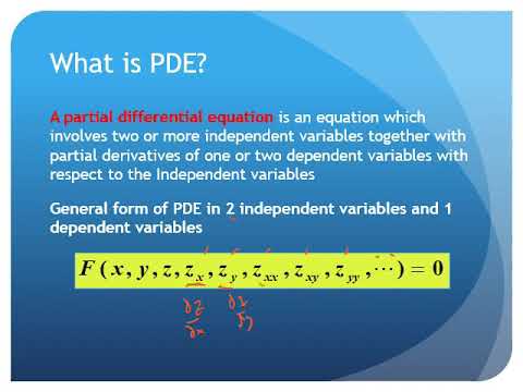
What are partial differential equations and how do they differ from ordinary differential equations?

Partial differential equations (PDEs) involve partial derivatives and have multiple variables, unlike ordinary differential equations (ODEs) which typically involve a single independent variable. PDEs are used to describe phenomena in multiple dimensions, such as heat conduction or wave propagation.

What are the goals for the end of the series mentioned in the script?

The goals for the end of the series are to reach and explain partial differential equations, including the heat equation, wave equation, and possibly the Laplace equation, providing a comprehensive understanding of differential equations beyond the basics.

Outlines

00:00

📚 Introduction to Ordinary Differential Equations

The video script introduces the concept of ordinary differential equations (ODEs), focusing on first and second order equations which are most commonly encountered in applications. It explains the significance of first order equations involving first derivatives, which represent the rate of change of an unknown function y with respect to time. The script also touches on the idea of inputs, or forcing terms, that can cause the solution to grow, decay, or oscillate. The distinction between linear and nonlinear equations is made, with the former being more solvable in certain cases. The video promises a deep dive into these equations, including their applications and the challenges they present.

05:03

🔍 Exploring Linear and Nonlinear Second Order Equations

This paragraph delves into the specifics of second order ODEs, which involve second derivatives and can represent acceleration or the bending of a graph. It discusses the importance of linearity and constant coefficients in solving these equations, and how solutions can be represented by exponential functions. The script also mentions the challenges of solving equations with non-constant coefficients and nonlinearities, which often require numerical methods. The concept of systems of equations is introduced, where multiple equations are coupled, and the role of eigenvalues and eigenvectors in simplifying these systems is highlighted. The paragraph concludes with an overview of numerical solutions and the use of MATLAB for solving ODEs.

10:04

🌐 Transition to Systems of Equations and Numerical Methods

The final paragraph of the script discusses the transition from single equations to systems of equations, which are common in real-world applications. It explains how these systems can be represented as matrices and how linear algebra concepts like eigenvalues and eigenvectors can be used to decouple them into simpler, solvable equations. The paragraph also emphasizes the prevalence of numerical solutions in the field of ODEs, especially with the use of software like MATLAB. It mentions the ODE solvers available in MATLAB, starting with the basic Euler method and progressing to the more advanced and accurate ODE45. The script sets a goal to eventually cover partial differential equations (PDEs), highlighting the heat, wave, and Laplace equations as part of the broader scope of the series.

Keywords

💡Ordinary Differential Equations (ODEs)

Ordinary Differential Equations, or ODEs, are equations that involve ordinary derivatives, which are derivatives with respect to a single independent variable. In the context of the video, ODEs are the primary focus, as they are essential for understanding the changes in functions over time. The script discusses both first and second order ODEs, highlighting their applications in various fields such as physics and engineering.

💡First Order Equations

First order equations are a type of differential equation that involve the first derivative of the function. They are fundamental to the video's theme as they represent the rate of change of a function and are often solvable, especially when they are linear. The script mentions that these equations can model scenarios like the growth or decay of a quantity, such as money in a bank account.

💡Second Order Equations

Second order equations involve the second derivative of a function, which typically represents acceleration in physical systems. The video script emphasizes the importance of second order equations in modeling the bending or curvature of a function's graph, and their role in understanding phenomena described by Newton's laws of motion.

💡Derivative

A derivative in calculus represents the rate at which a quantity changes with respect to another quantity. In the video, the derivative is used to describe the rate of change of an unknown function 'y' with respect to time, which is central to the concept of differential equations.

💡Linear Equations

Linear equations are those in which the variable and its derivatives appear to the first power only. The script explains that linearity simplifies the process of finding solutions to differential equations, as it allows for the separation of variables and the application of standard techniques.

💡Nonlinear Equations

Nonlinear equations are those where the variable or its derivatives appear in a power higher than one or are involved in a function that is not a polynomial. The video script points out that nonlinear equations can be more challenging to solve and may require numerical methods or special functions.

💡Forcing Term

A forcing term in a differential equation represents an external input that influences the behavior of the system. In the script, it is mentioned that this term can cause the solution to grow, decay, or oscillate, and is crucial in understanding the system's response to external influences.

💡Eigenvalues and Eigenvectors

Eigenvalues and eigenvectors are concepts from linear algebra that are used to solve systems of linear equations. The video script introduces these terms in the context of solving systems of differential equations, where they can simplify the process by transforming coupled equations into simpler, uncoupled ones.

💡Numerical Solutions

Numerical solutions refer to the approximate solutions obtained through computational methods when analytical solutions are not feasible. The script mentions that a significant part of the subject matter involves finding numerical solutions to differential equations, especially when dealing with nonlinear or complex systems.

💡MATLAB

MATLAB is a programming environment and language widely used for numerical computing, including the solution of differential equations. The video script highlights MATLAB's ODE solvers, such as ODE45, which are essential tools for obtaining numerical solutions to ODEs.

💡Partial Differential Equations (PDEs)

Partial Differential Equations involve partial derivatives and are used to describe phenomena involving multiple independent variables. The script sets a goal to eventually cover PDEs, such as the heat equation and wave equation, which are fundamental in fields like physics and engineering.

Highlights

Introduction to ordinary differential equations and their applications.

Focus on first and second order differential equations due to their prevalence and solvability.

First order equations involve first derivatives, representing the rate of change of the unknown function.

Differential equations connect changes in the function with its current state.

Linear equations with a forcing term are discussed, illustrating how inputs affect the system.

Nonlinear equations are introduced, where the derivative's value depends on the function itself.

General first order equations may depend on both time and the function, with inputs varying over time.

Second order equations involve second derivatives, indicating acceleration and curve bending.

Newton's law is used to explain the relationship between force, mass, acceleration, and damping.

The importance of linearity and constant coefficients in solving second order equations is emphasized.

Solutions to differential equations are often exponential functions, which are repeatedly encountered.

Some solutions may involve integrals of the function, requiring lookup or numerical methods.

Nonlinear functions and varying coefficients typically require numerical solutions.

Systems of equations are introduced, where multiple equations are coupled, represented by a matrix.

Eigenvalues and eigenvectors are key to simplifying systems of equations by decoupling them.

Numerical solutions are the predominant method for finding solutions in practice, with MATLAB being a leading tool.

Cleve Moler's series on MATLAB for numerical solutions, starting with Euler's method and advancing to ODE 45.

The goal of the series is to provide a clear understanding of basic differential equations that can be solved and comprehended.

Partial differential equations are mentioned as a future topic, including the heat, wave, and Laplace equations.

Transcripts

GILBERT STRANG: OK.

Well, the idea of this first video

is to tell you what's coming, to give a kind of outline

of what is reasonable to learn about ordinary differential

equations.

And a big part of the series will

be videos on first order equations and videos

on second order equations.

Those are the ones you see most in applications.

And those are the ones you can understand and solve,

when you're fortunate.

So first order equations means first derivatives

come into the equation.

So that's a nice equation that we will solve,

we'll spend a lot of time on.

The derivative is-- that's the rate of change of y--

the changes in the unknown y-- as time goes forward

are partly from depending on the solution itself.

That's the idea of a differential equation,

that it connects the changes with the function y as it is.

And then you have inputs called q of t,

which produce their own change.

They go into the system.

They become part of y.

And they grow, decay, oscillate, whatever y of t does.

So that is a linear equation with a right-hand side,

with an input, a forcing term.

And here is a nonlinear equation.

The derivative of y.

The slope depends on y.

So it's a differential equation.

But f of y could be y squared over y cubed or the sine of y

or the exponential of y.

So it could be not linear.

Linear means that we see y by itself.

Here we won't.

Well, we'll come pretty close to getting

a solution, because it's a first order equation.

And the most general first order equation, the function

would depend on t and y.

The input would change with time.

Here, the input depends only on the current value of y.

I might think of y as money in a bank,

growing, decaying, oscillating.

Or I might think of y as the distance on a spring.

Lots of applications coming.

OK.

So those are first order equations.

And second order have second derivatives.

The second derivative is the acceleration.

It tells you about the bending of the curve.

If I have a graph, the first derivative we know

gives the slope of the graph.

Is it going up?

Is it going down?

Is it a maximum?

The second derivative tells you the bending of the graph.

How it goes away from a straight line.

So and that's acceleration.

So Newton's law-- the physics we all live with--

would be acceleration is some force.

And there is a force that depends, again, linearly--

that's a keyword-- on y.

Just y to the first power.

And here is a little bit more general equation.

In Newton's law, the acceleration

is multiplied by the mass.

So this includes a physical constant here, the mass.

Then there could be some damping.

If I have motion, there may be friction slowing it down.

That depends on the first derivative, the velocity.

And then there could be the same kind of forced term

that depends on y itself.

And there could be some outside force, some person or machine

that's creating movement.

An external forcing term.

So that's a big equation.

And let me just say, at this point,

we let things be nonlinear.

And we had a pretty good chance.

If we get these to be non-linear,

the chance at second order has dropped.

And the further we go, the more we

need linearity and maybe even constant coefficients.

m, b, and k.

So that's really the problem that we

can solve as we get good at it is a linear equation--

second order, let's say-- with constant coefficients.

But that's pretty much pushing what

we can hope to do explicitly and really

understand the solution, because so

linear with constant coefficients.

Say it again.

That's the good equations.

And I think of solutions in two ways.

If I have a really nice function like a exponential.

Exponentials are the great functions

of differential equations, the great functions in this series.

You'll see them over and over.

Exponentials.

Say f of t equals-- e to the t.

Or e to the omega t.

Or e to the i omega t.

That i is the square root of minus 1.

In those cases, we will get a similarly nice function

for the solution.

Those are the best.

We get a function that we know like exponentials.

And we get solutions that we know.

Second best are we get some function we don't especially

know.

In that case, the solution probably

involves an integral of f, or two integrals of f.

We have a formula for it.

That formula includes an integration

that we would have to do, either look it up

or do it numerically.

And then when we get to completely non-linear

functions, or we have varying coefficients,

then we're going to go numerically.

So really, the wide, wide part of the subject

ends up as numerical solutions.

But you've got a whole bunch of videos

coming that have nice functions and nice solutions.

OK.

So that's first order and second order.

Now there's more, because a system doesn't usually

consist of just a single resistor or a single spring.

In reality, we have many equations.

And we need to deal with those.

So y is now a vector.

y1, y2, to yn.

n different unknowns.

n different equations.

That's n equation.

So here that is an n by n matrix.

So it's first order.

Constant coefficient.

So we'll be able to get somewhere.

But it's a system of n coupled equations.

And so is this one with a second derivative.

Second derivative of the solution.

But again, y1 to yn.

And we have a matrix, usually a symmetric matrix

there, we hope, multiplying y.

So again, linear.

Constant coefficients.

But several equations at once.

And that will bring in the idea of eigenvalues

and eigenvectors.

Eigenvalues and eigenvectors is a key bit of linear algebra

that makes these problems simple,

because it turns this coupled problem

into n uncoupled problems.

n first order equations that we can solve separately.

Or n second order equations that we can solve separately.

That's the goal with matrices is to uncouple them.

OK.

And then really the big reality of this subject

is that solutions are found numerically

and very efficiently.

And there's a lot to learn about that, a lot to learn.

And MATLAB is a first-class package

that gives you numerical solutions with many options.

One of the options may be the favorite.

ODE for ordinary differential equations 4 5.

And that is numbers 4, 5.

Well, Cleve Moler, who wrote the package MATLAB,

is going to create a series of parallel videos

explaining the steps toward numerical solution.

Those steps begin with a very simple method.

Maybe I'll put the creator's name down.

Euler.

So you can know that because Euler was centuries ago,

he didn't have a computer.

But he had a simple way of approximating.

So Euler might be ODE 1.

And now we've left Euler behind.

Euler is fine, but not sufficiently accurate.

ODE 45, that 4 and 5 indicate a much higher accuracy, much more

flexibility in that package.

So starting with Euler, Cleve Moler

will explain several steps that reach

a really workhorse package.

So that's a parallel series where you'll see the codes.

This will be a chalk and blackboard

series, where I'll find solutions in exponential form.

And if I can, I would like to conclude the series by reaching

partial differential equations.

So I'll just write some partial differential equations here,

so you know what they mean.

And that's a goal which I hope to reach.

So one partial differential equation

would be du dt-- you see partial derivatives-- is

second derivative.

So I have two variables now.

Time, which I always have.

And here is x in the space direction.

That's called the heat equation.

That's a very important constant coefficient,

partial differential equation.

So PDE, as distinct from ODE.

And so I write down one more.

The second derivative of u is the same right-hand side

second derivative in the x direction.

That would be called the wave equation.

So this is like the first order equation in time.

It's like a big system.

In fact, it's like an infinite size system of equations.

First order in time.

Or second order in time.

Heat equation.

Wave equation.

And I would like to also include a the Laplace equation.

Well, if we get there.

So those are goals for the end of the series that

go beyond some courses in ODEs.

But the main goal here is to give you

the standard clear picture of the basic differential

equations that we can solve and understand.

Well, I hope it goes well.

Thanks.