Understanding the Finite Element Method

Summary

This video delves into the finite element method, a crucial tool in engineering for solving complex structural mechanics problems. It explains how this numerical technique breaks down a body into smaller elements, creating a mesh to simplify equilibrium calculations. The script covers element types, degrees of freedom, and stiffness matrices, highlighting the process from problem definition to post-processing. It also touches on the derivation of stiffness matrices and the role of software in handling complex calculations, providing a foundational understanding of this powerful analysis method.

Takeaways

• 🔍 The finite element method (FEM) is a numerical technique used by engineers to solve complex structural and mechanics problems that cannot be easily solved analytically.
• 🌐 FEM is widely applied across major engineering industries for various analyses, including static, dynamic, buckling, modal, fluid flow, heat transfer, and electromagnetic problems.
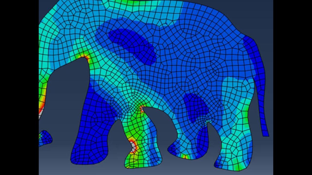
• 🛠️ The method involves breaking down a complex structure into smaller, simpler elements connected at nodes, creating a 'mesh' that can be analyzed for equilibrium.
• 📐 FEM allows for the calculation of 'field variables' such as stresses, strains, and displacements within a structure under load.
• 📊 Different element shapes like triangular, quadrilateral, solid, and line elements can be used in FEM, chosen based on the specific analysis requirements and the geometry of the structure.
• 🔗 The stiffness matrix, derived from Hooke's law, is crucial for FEM as it relates the nodal forces and moments to the nodal displacements within each element.
• 🧩 The global stiffness matrix is assembled from individual element stiffness matrices, considering the connectivity and continuity of the elements in the mesh.
• 🔄 FEM involves iterative processes for solving the global stiffness matrix, often using methods like the conjugate gradient method due to the large size and sparse nature of the matrix.
• 📉 Post-processing of the nodal displacements obtained from FEM allows for the calculation of secondary outputs such as stress and strain throughout the structure.
• 🔧 Engineers play a critical role in FEM by defining the problem, selecting appropriate element types, ensuring a suitable mesh, and validating the results for accuracy and reliability.

Q & A

What is the finite element method and why is it important in engineering?

The finite element method is a powerful numerical technique that uses computational power to calculate approximate solutions to complex structural mechanics problems. It's important in engineering because it allows for the analysis of complex geometries, loads, or materials that cannot be solved using traditional analytical methods.

How does the finite element method handle complex problems that traditional analytical methods cannot solve?

The finite element method handles complex problems by discretizing the body into small elements connected at nodes, allowing the equilibrium requirement to be satisfied over a finite number of discrete elements instead of continuously over the entire body.

What are the different types of elements used in the finite element method?

Different types of elements used include triangular and quadrilateral surface elements for modeling thin surfaces, solid elements for three-dimensional bodies, and line elements. The choice of element depends on the specific scenario being analyzed and requires expertise.

Why is the concept of equilibrium important in the finite element method?

The concept of equilibrium is important because internal stresses within a body develop to maintain equilibrium over any volume of the body. This concept is used to calculate field variables such as stresses, strains, and displacements within the body.

What is a degree of freedom in the context of the finite element method?

A degree of freedom in the finite element method refers to the number of independent displacement components possible at a node. For example, in a two-dimensional case with beam elements, each node can translate along the X and Y axes and rotate about the Z axis, resulting in three degrees of freedom per node.

How is the stiffness matrix of an element derived in the finite element method?

The stiffness matrix of an element is derived by enforcing equilibrium and can be obtained through various methods such as the direct method, the principle of minimum potential energy, or the Galerkin method of weighted residuals. These methods help define how much each node in the element will displace for a set of forces and moments applied to the nodes.

What is the significance of the global stiffness matrix in the finite element method?

The global stiffness matrix is significant because it defines how the entire structure will displace when loads are applied. It is assembled from individual element stiffness matrices based on how the elements are connected together, and it is used to solve for the displacements at each node in the structure.

How are boundary conditions applied in the finite element method?

Boundary conditions in the finite element method are applied by defining known displacements at specific nodes, typically because certain degrees of freedom are fixed. These conditions are used to solve the global stiffness matrix equation to obtain the displacements at each node.

What is the role of software in the finite element method?

Software plays a crucial role in the finite element method by automating complex calculations such as deriving element stiffness matrices, assembling the global stiffness matrix, and solving the model. It also aids in post-processing to obtain results and validating the model, which would be impossible to do manually for complex models.

How does the finite element method account for different material properties and loads?

The finite element method accounts for different material properties and loads by incorporating these factors into the element stiffness matrix calculations. The material properties affect the element's resistance to deformation, while the loads determine the forces and moments applied to the nodes.

What is the purpose of shape functions in the finite element method?

Shape functions in the finite element method are used to describe how displacements and other field variables vary inside the element. They are usually polynomial assumptions that interpolate values at the nodes to calculate values within the element, which is necessary for methods like the Galerkin method.

Outlines

00:00

🔍 Introduction to Finite Element Method

This paragraph introduces the finite element method (FEM) as a powerful numerical technique used by engineers to solve complex structural and mechanics problems. It highlights the versatility of FEM in various industries, such as aerospace and automotive, for tasks like ensuring satellite components' durability during launch or optimizing car suspension designs. The FEM is particularly useful for static, dynamic, buckling, and modal analyses in solid mechanics, as well as for fluid flow, heat transfer, and electromagnetic problems. The focus of this introduction is on static, linear-elastic stress analysis, exemplified by analyzing the stress on an air conditioning unit's supporting bracket. The concept of 'field variables' like stresses, strains, and displacements is introduced, along with the importance of equilibrium in calculating these variables. The FEM approach involves discretizing the body into small elements connected at nodes, forming a 'mesh,' which simplifies the equilibrium requirement to discrete elements rather than the entire body. Different element shapes like triangular and quadrilateral surface elements, solid elements, and line elements are mentioned, each suitable for specific scenarios and offering varying levels of accuracy and performance.

05:02

🔧 Element Stiffness and Degrees of Freedom

This paragraph delves into the concept of element stiffness and degrees of freedom in the finite element method. It explains how each node in a mesh can experience different types of displacements, such as translation and rotation, which are referred to as degrees of freedom. The paragraph contrasts the degrees of freedom for 2D and 3D elements, highlighting that 3D elements have more complex requirements. It introduces the idea of element stiffness, analogous to a spring's resistance to deformation, and how it is represented mathematically through a stiffness matrix. The stiffness matrix is crucial for calculating nodal displacements within the mesh and is derived by enforcing equilibrium within each element. The paragraph also discusses how individual element stiffness matrices are assembled into a global stiffness matrix, which defines the entire structure's response to applied loads. The assembly process considers the connectivity of elements and ensures continuity at shared nodes. The characteristics of the global stiffness matrix, such as sparsity, banding, and symmetry, are also described. Finally, the paragraph touches on the need to apply boundary conditions and external loads to solve for nodal displacements using the global stiffness matrix, which can be achieved through various numerical methods like the conjugate gradient method.

10:05

🧩 Assembling the Global Stiffness Matrix and Solving the Model

The third paragraph continues the discussion on the finite element method by focusing on the assembly of the global stiffness matrix and the process of solving the model. It emphasizes the importance of aligning element stiffness matrices with a global coordinate system, which may require transformation using rotation matrices. The paragraph describes how the global stiffness matrix, once assembled, is used in conjunction with boundary conditions and external loads to calculate the displacements at each node within the structure. It mentions that solving the global stiffness matrix equation is typically done using iterative methods rather than matrix inversion, due to the matrix's sparsity and size. The paragraph also outlines the subsequent steps of calculating strains and stresses throughout the mesh once nodal displacements are known. It concludes by emphasizing the role of software in handling complex calculations and the engineer's responsibility in problem definition, mesh suitability, and result validation.

15:07

🔬 Derivation of Stiffness Matrices and Overview of the Finite Element Method

The final paragraph of the script returns to the derivation of stiffness matrices for various element types, explaining different methods based on equilibrium concepts. It contrasts the 'strong' form of equilibrium problems, which are directly solved using differential equations, with the 'weak' forms that offer approximate solutions and are easier to handle. The paragraph introduces two weak form methods: the Principle of Minimum Potential Energy and the Galerkin method of weighted residuals, both of which are used to derive stiffness matrices. The importance of shape functions for interpolating values within elements is also highlighted. The paragraph summarizes the finite element method process, which includes defining the problem, discretizing the body, defining element stiffness matrices, assembling the global stiffness matrix, solving for nodal displacements, calculating stresses and strains, and finally, post-processing and validating the model. It concludes by encouraging viewers to explore further through extended content on Nebula and promoting CuriosityStream as a platform for curious minds, offering a discount and access to Nebula as part of the subscription.

Keywords

💡Finite Element Method (FEM)

The Finite Element Method is a numerical technique used by engineers to solve complex structural and mechanical problems that cannot be easily solved analytically. It involves breaking down a complex structure into smaller, simpler elements, which can then be analyzed computationally. In the video, FEM is used to illustrate how to calculate stresses, strains, and displacements in structures like satellite components and automotive parts. It's a core theme as it's the main method being discussed and demonstrated.

💡Discretisation

Discretisation is the process of dividing a continuous system or structure into discrete elements, which is a fundamental step in the Finite Element Method. It allows for the application of numerical methods to solve problems that would be intractable when considering the system as a whole. In the script, discretisation is used to simplify the analysis of complex geometries by creating a mesh of elements connected at nodes.

💡Mesh

A mesh in the context of FEM refers to the collection of nodes and elements that discretise the geometry of the structure being analyzed. It is a representation of the physical model that is used for computational analysis. The script mentions that the equilibrium requirement only needs to be satisfied over these discrete elements, making the problem more manageable.

💡Degrees of Freedom (DOF)

Degrees of Freedom in FEM refer to the number of independent displacements or rotations that a node within a mesh can have. Each DOF represents a direction in which a node can move or rotate. The script explains that for a 2D beam element, there are typically three DOFs per node, allowing for translation in two axes and rotation about one axis.

💡Stiffness Matrix

The stiffness matrix is a key component in FEM that relates the forces and displacements within an element. It quantifies the resistance of an element to deformation and is used to assemble the global stiffness matrix for the entire structure. The script provides an example of how the stiffness matrix for a 2D beam element looks and how it is derived from equilibrium equations.

💡Equilibrium

Equilibrium in mechanics refers to the state where the sum of all forces and moments acting on a body is zero, resulting in no net motion. In FEM, enforcing equilibrium at the element level is crucial for calculating field variables like stresses and displacements. The script discusses how equilibrium is applied to calculate the bending moment and shear force in a beam, which are then used to determine stresses.

💡Global Stiffness Matrix

The global stiffness matrix is an assembly of individual element stiffness matrices that represents the overall stiffness of the entire structure in FEM. It is used to solve for the nodal displacements when external loads are applied. The script explains how element matrices are assembled into a global matrix based on how the elements are connected within the mesh.

💡Boundary Conditions

Boundary conditions in FEM define the constraints or known displacements at certain nodes of the mesh. They are essential for solving the system as they provide the necessary information to determine the unknown displacements. The script mentions boundary conditions as fixed displacements at specific nodes, which are crucial for solving the global stiffness matrix.

💡Element Types

Element types refer to the different shapes and formulations used to model parts of a structure in FEM. The choice of element type depends on the geometry and the loading conditions of the problem. The script discusses various element types such as surface elements, solid elements, and line elements, each with specific applications and formulations.

💡Post-processing

Post-processing in FEM involves analyzing and interpreting the results obtained from the numerical solution, such as displacements, stresses, and strains. It is the final step where the engineer extracts meaningful information from the data. The script briefly mentions post-processing as a step after solving for nodal displacements to obtain the desired results.

Highlights

The finite element method is a powerful numerical technique used for solving complex structural mechanics problems.

It's widely used in major engineering industries for various applications, including satellite and automotive component analysis.

The method allows for the analysis of solid mechanics problems such as static, dynamic, buckling, and modal analyses.

It can also address fluid flow, heat transfer, and electromagnetic problems.

The focus of this introduction is on static, linear-elastic stress analysis using the finite element method.

The goal of static stress analysis is to calculate stresses, strains, and displacements within a structure.

The finite element method involves discretisation of the body into small elements connected at nodes, forming a mesh.

Different element shapes like triangular, quadrilateral, solid, and line elements can be used depending on the problem's complexity.

The choice of element type requires expertise and depends on the specific scenario being analysed.

The fundamental variable for stress analysis problems is the displacement at each node.

Each element can be defined by a vector {u} that contains all possible displacements for its nodes, including rotations.

The stiffness matrix [k] of an element is key to solving the displacements at every node of the mesh.

The global stiffness matrix is assembled from individual element stiffness matrices based on how elements are connected.

Boundary conditions and external loads must be defined to solve for nodal displacements.

Commercial solvers use iterative methods like the conjugate gradient method to solve the global stiffness matrix.

Once nodal displacements are found, strains and stresses throughout the mesh can be calculated.

The finite element method requires appropriate software for complex models with a high number of degrees of freedom.

Stiffness matrices can be derived using the direct method, variational principles, or the Galerkin method.

Shape functions are used to describe how displacements and field variables vary inside the element.

The finite element method involves defining the problem, discretisation, stiffness matrix definition, assembly into a global matrix, and solving for displacements.

Post-processing and validation of the model are crucial steps after solving for displacements.

Transcripts

Thanks to CuriosityStream for sponsoring this video.

There are a lot of different analytical methods that engineers can use to solve structural

mechanics problems, whether it's to calculate the deflection of a beam or the stresses in

a flat plate.

But we often encounter problems that can't be solved in this way, typically because the

geometry, loads or materials are too complex.

The finite element method is a powerful numerical technique that uses computational

power to calculate approximate solutions to these types of problems.

It's widely used in all major engineering industries.

It could be used to check that satellite components will survive the launch conditions, for example.

Or to optimise the design of automotive components, like the lower control arm of this car's suspension

system.

Finite element analysis software can be used to analyse a wide range of solid mechanics

problems, including static, dynamic, buckling, and modal analyses.

But it can also be used for fluid flow, heat transfer, and electromagnetic problems.

For this introduction to the finite element method, we'll focus on how it applies to static

linear-elastic stress analysis.

Imagine we want to analyse the brackets supporting this air conditioning unit.

The goal of a static stress analysis would typically be to calculate the stresses, strains

and displacements within the bracket.

These unknowns are called "field variables".

Internal stresses develop within a body in such a way as to maintain equilibrium over

any volume of the body, so we can apply the concept of equilibrium to calculate the field

variables.

This is easy to do for a simple beam - we can use equilibrium to calculate the bending

moment and shear force along it, and from there we can calculate the normal and shear

stresses in the beam.

But enforcing equilibrium over a two dimensional shape like this bracket is difficult, and

it becomes even more complicated for a three dimensional body.

The finite element method approaches this problem by splitting the body into a number

of small elements, that are connected together at nodes.

This process is called discretisation, and the collection of nodes and elements is called

the mesh.

Discretisation is useful because the equilibrium requirement now only needs to be satisfied

over a finite number of discrete elements, instead of continuously over the entire body.

Several different element shapes can be used.

We've used triangular surface elements to model this bracket.

Surface elements are two dimensional elements that are typically used to model thin surfaces.

They can be triangular or quadrilateral.

Triangular elements are good for modelling awkward shapes, although quadrilateral elements

tend to perform better.

Solid elements are used for three-dimensional bodies.

And then we have line elements.

Choosing the right element for your model will depend on the specific scenario being

analysed, and requires some expertise.

In the case of our bracket we could have used solid elements, or even line elements, depending

on how much we wanted to simplify the problem.

Even for elements of the same shape, there are hundreds of different types to choose

from that each have different formulations, and introduce different levels of approximation.

A line element can be a bar, for example, that only carries axial loads, or a beam,

that can carry axial, bending, shear and torsional loads.

We can model the bracket using plane stress surface elements, because the bracket is thin

and the loading is all in the same plane.

But that's only one of many surface element types.

These are all first order elements, but we can also use second order elements, which

have additional mid-side nodes and are more accurate.

For stress analysis problems the fundamental variable we want to calculate is the displacement

at each node.

If we know how a body displaces when loads are applied, we'll easily be able to calculate

secondary outputs like stress and strain.

For each element we can define a vector {u} that contains all of the possible displacements

for the nodes of the element, including rotations.

If we're analysing a two-dimensional case with beam elements, each node can translate

along the X and Y axes and it can rotate about the Z axis, so the vector {u} will look like

this.

Each of these displacements is called a degree of freedom.

For the beam element we have 3 degrees of freedom per node, or 6 in total.

For a 3D case that increases to 6 degrees of freedom per node.

A shell element node also has 3 degrees of freedom in two dimensions, but since the element

has 4 nodes, it has 12 degrees of freedom in total.

The nodes of a solid element only have the 3 translational degrees of freedom.

The nodes aren't allowed to rotate and instead rotation of the element is captured by translation

of the nodes.

So how can we calculate all of the displacements at every node in our mesh?

For a spring, the relationship between force and displacement is defined by Hooke's law.

The spring stiffness k determines how far the spring will displace for a given force.

In the same way, we can think of the elements of our mesh as having a certain amount of

stiffness, that resists deformation.

In this equation {f} is a vector of the nodal forces and moments, {u} is the vector of the

nodal displacements, and [k] is the stiffness matrix of the element.

A 2D beam element has 6 degrees of freedom, so the displacement vector looks like this.

And the force vector and the stiffness matrix will look like this.

The element stiffness matrix defines how much each node in the element will displace for

a set of forces and moments applied to the nodes, and so is the key to solving the displacements

at every node of our mesh.

It's a square matrix - the number of rows and the number of columns are equal to the

number of degrees of freedom of the element.

We can figure out what the terms of the stiffness matrix are by enforcing equilibrium.

We'll come back to this later on in the video, but for a 2D beam the matrix looks like this.

We can think of this equation as a system of linear equations that we can solve to obtain

the displacements at the nodes of our mesh.

If we apply a lateral displacement to node 2, for example, and all of the other degrees

of freedom are fixed, and so are equal to zero, we can use the stiffness matrix to calculate

the forces and moments at both of the nodes.

To make the next steps easier to visualise, let's represent the stiffness matrix in a

more abstract form.

This is just one element, but our overall mesh will be made up of many more elements.

Let's look at a simple example where we have a mesh made up of three 2D beam elements,

that we're using to model a cantilever beam.

We can assemble the individual stiffness matrices for all of the elements in our mesh into a

huge global stiffness matrix that defines how the entire structure will displace when

loads are applied to it.

Like the element stiffness matrix, the global stiffness matrix is a square matrix and the

number of rows and columns is equal to the total number of degrees of freedom in the

model.

The element stiffness matrices are assembled together to form the global stiffness matrix

based on how the elements are connected together.

Elements 1 and 2 are connected at node 2 for example.

Continuity tells us that since these two elements are connected at the same node, the displacements

for both elements must be the same at the common node.

So when we assemble the global stiffness matrix, the terms in the element stiffness matrices

corresponding to node 2 should be summed for each degree of freedom.

Element 3 is not connected to node 2, so this element's stiffness matrix should have no

effect on the displacements at node 2.

This is what the actual global stiffness matrix looks like for this model.

It has some interesting characteristics.

It is said to be sparse, because it contains a lot of zeros, and banded, because the non-zero

terms are grouped around the diagonal.

For linear-elastic problems the matrix will also be symmetric.

If we modify the mesh so that the three elements are connected differently, the global stiffness

matrix will change.

In this case we have three nodes instead of four, so the matrix will be smaller, and the

fact that elements 1 and 3 are connected is reflected in the matrix.

An important thing to note here is that the elements are no longer aligned to the same

coordinate system, so we have to transform the stiffness matrix for each element so that

it aligns with a global coordinate system.

We can do this by multiplying each element stiffness matrix by a rotation matrix.

Now that we've assembled the global stiffness matrix, we need to solve this equation to

obtain the displacements at each of the nodes.

To do this we need to define the external loads, and the boundary conditions.

The boundary conditions are known displacements at specific nodes, typically because specific

degrees of freedom are fixed.

In this model, vertical and horizontal translations are fixed at node 1, and vertical translations

are fixed at node 2, so the displacement vector looks like this.

And the force vector will look like this.

It includes the applied force and the reaction forces at the supports.

Now we can solve the equation.

We could do this by inverting the global stiffness matrix and solving the displacements from

there.

But in practice inverting the matrix isn't very efficient, particularly because it's

a sparse matrix.

Commercial solvers mostly use methods that involve iteratively approximating the displacement

vector, like the conjugate gradient method.

Once we've solved for the nodal displacements, we can calculate the strains and then stresses

throughout the mesh.

A typical finite element mesh could easily have a hundred thousand degrees of freedom,

which would be impossible to solve by hand, and so applying the finite element method

to anything more complicated than a very basic model requires the use of appropriate software.

Now that we have an overall understanding of the finite element method, let's return

to the element stiffness matrix to see how it's derived.

The matrix shown here is for a 2D beam element, but it will look very different for different

element types.

Several different methods can be used to derive these stiffness matrices, and they are all

fundamentally based on the concept of equilibrium.

The direct method derives the stiffness matrix directly from the equilibrium equations that

govern the behaviour of the element.

The lateral deflection of a beam is governed by this equation, for example, so we can solve

the equation to obtain the stiffness matrix for a beam element.

These governing equations are usually differential equations.

The differential equations and associated boundary conditions are what we call the "strong"

form of the equilibrium problem.

But it's only really possible to solve the strong form for simple elements.

For more general cases we can use "weak" forms that describe the differential equations in

integral form, instead of solving the differential equations directly.

These give approximate solutions to the equilibrium equations, but are easier to solve.

The first of the weak form methods is based on variational principles.

One such principle commonly used for structural mechanics problems is the Principle of Minimum

Potential Energy.

It states that the displacement configuration that satisfies equilibrium conditions is the

one that minimises the total potential energy, where the potential energy is the sum of the

strain energy and the potential energy of the external loads.

By applying a mathematical technique called the calculus of variations to minimise the

total potential energy, we can obtain an approximate solution to the equilibrium equations.

The other weak form method is the Galerkin method of weighted residuals.

In this method the function that satisfies the differential equation is approximated

as the sum of a number of assumed trial functions that each have unknown coefficients.

This approximate solution is substituted into the differential equation, and an equation

for the error, called the residual, is obtained.

If we multiply each trial function by the residual and set the integral of this product

to zero, we can calculate the unknown coefficients that minimise the residual.

This gives us an approximate solution to the differential equation.

This is a more widely applicable approach than the principle of minimum potential energy,

but for stress analysis problems both methods give the same result.

Regardless of which method we use, we end up with the stiffness matrix for our element.

But to apply these methods we need to be able to describe how displacements and other field

variables vary inside the element, instead of just at the nodes of the element.

To overcome this issue, an element needs to have a defined function that calculates values

inside the element by interpolating the values at the nodes.

The shape function is just an assumption.

It's usually chosen to be a polynomial, since they're relatively simple and sufficiently

accurate.

And with that we've covered all of the key aspects of the finite element method.

In summary, the first step in the finite element method is defining the problem, including

the relevant material properties, loads and boundary conditions.

Next the body being analysed is split into a number of small elements connected at nodes,

and the element types are chosen.

Then a stiffness matrix is defined for each element, using one of the three methods we

covered earlier.

The element stiffness matrices are then assembled into a global stiffness matrix based on element

connectivity.

This global stiffness matrix defines how the structure will respond to applied loads, and

we can use it along with boundary conditions to solve for the displacement at each node

in the structure.

Once we have displacements we can calculate stresses, strains and other field variables

of interest.

Then all that's left to do is post-processing to obtain the desired results, and validation

of the model.

A lot of the hard work like calculating the element stiffness matrices, assembling the

global stiffness matrix and solving the model is done by the software being used.

But the engineer is responsible for making sure that the problem has been properly defined,

that the mesh is suitable, and for interpreting and validating the results.

I hope this video has helped you develop a better understanding of the fundamentals of

the finite element method.

If you're interested in learning more, you can check out the extended version of this

video, that's available now over on Nebula, where I spend a few more minutes covering

the problem definition, discretisation, post-processing, and validation steps.

Nebula is a streaming service built by independent educational creators.

It's a place where you can find extended versions of my videos, alongside amazing original content

from other creators, like Mustard and Wendover, without any ads or sponsor messages.

You can get access to Nebula for free when you sign up for CuriosityStream.

CuriosityStream is the perfect streaming service for curious minds.

It has thousands of high quality documentaries to keep you entertained and learning, like

Particle Fever, an incredible film that follows experimental and theoretical physicists during

the first round of experiments at the Large Hadron Collider, the largest science experiment

ever conducted, as they work to prove the existence of the Higgs boson particle.

If you sign up to CuriosityStream using this link, you'll get a 26% discount on their annual

plan, and you'll get access to Nebula for free.

All for less than $15 a year.

So to watch my bonus content on Nebula, and Particle Fever and countless other documentaries

on CuriosityStream, head over to curiositystream.com/efficientengineer, or click the link in the description.

It's an amazing deal, and signing up is a great way to support this channel.

And that's it for this introduction to the finite element method.

Thanks for watching!