Derive Time Independent SCHRODINGER's EQUATION from Time Dependent one
Summary
TLDRIn this educational video, the presenter demonstrates how to transform the time-dependent Schrödinger equation into its time-independent form using the separation of variables method. This technique is crucial in quantum mechanics for analyzing the behavior of particles under potential fields that are time-independent. The video elucidates the process of reducing a complex partial differential equation to a simpler ordinary differential equation, which is essential for solving various quantum mechanical problems and understanding properties like energy levels and wavefunctions.
Takeaways
- 🔬 The video demonstrates the process of converting the time-dependent Schrödinger equation into its time-independent form using the separation of variables method.
- 🌌 In quantum mechanics, the Schrödinger equation is fundamental for studying the evolution of quantum systems, much like Newton's second law in classical mechanics.
- 📉 To use the separation of variables, the potential in the quantum system must be independent of time, allowing the wave function to be expressed as a product of spatial and temporal functions.
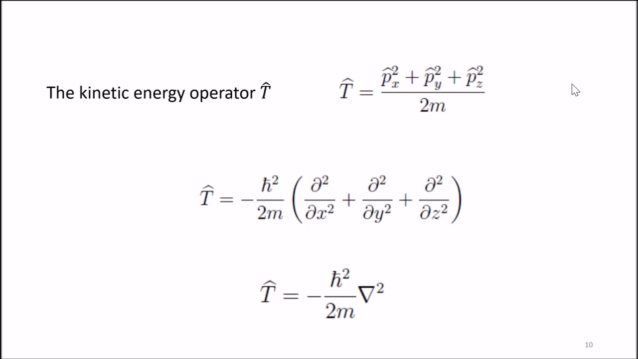
- ⏱️ The time-dependent Schrödinger equation is a partial differential equation involving both space and time derivatives, which can be simplified under the right conditions.
- 🧮 The reduction to an ordinary differential equation is achieved by assuming the wave function can be separated into functions of space and time, leading to two separate equations.
- 🔄 The separation constant, denoted as 'G', equates the spatial and temporal equations, suggesting that the energy of the system is related to the frequency of the time-dependent part of the wave function.
- 🌊 The time-independent part of the wave function is represented by a function of space only, which is crucial for solving the time-independent Schrödinger equation.
- 🌟 The solution to the time-independent equation provides eigenfunctions, which, when multiplied by the time-dependent part, give the complete wave function of the system.
- 📊 The probability density, derived from the wave function, remains constant over time for systems where the potential is time-independent, indicating stationary states.
- 🔍 The video concludes by emphasizing that the time-independent Schrödinger equation is essential for further analysis in quantum mechanical problems where the potential does not vary with time.
Q & A
What is the main topic of the video?
-The main topic of the video is the reduction of the time-dependent Schrödinger equation to its time-independent form using the separation of variables method.
Why is it important to study the trajectory of a quantum mechanical particle?
-Studying the trajectory of a quantum mechanical particle is important because it allows us to understand the evolution of the system, and from the solution of the Schrödinger equation, we can derive various physical quantities like position, momentum, velocity, and acceleration.
What is the fundamental equation in quantum mechanics that is discussed in the video?
-The fundamental equation in quantum mechanics discussed in the video is the Schrödinger equation.
How does the separation of variables method simplify the Schrödinger equation?
-The separation of variables method simplifies the Schrödinger equation by allowing the wave function to be expressed as a product of two separate functions, one dependent on space and the other on time, which reduces the partial differential equation to an ordinary differential equation.
Under what condition can the wave function be separated into space and time functions?
-The wave function can be separated into space and time functions when the potential field experienced by the particle is independent of time and only depends on the spatial variable.
What is the significance of the separation constant (G) in the context of the Schrödinger equation?
-The separation constant (G) in the Schrödinger equation is significant because it represents the energy of the particle in the quantum mechanical system, linking the frequency of the wave function to the energy of the particle through Planck's constant.
How is the time-independent Schrödinger equation derived from the time-dependent one?
-The time-independent Schrödinger equation is derived by separating the wave function into space and time components and setting the separated spatial and temporal parts equal to a constant, which leads to two ordinary differential equations, one for the spatial part and one for the temporal part.
What is the physical interpretation of the solution to the time-independent Schrödinger equation?
-The solution to the time-independent Schrödinger equation, often referred to as the eigenfunction, represents the spatial part of the wave function and is associated with the stationary states of the quantum system, where the probability density of the particle is constant over time.
Why are the solutions to the time-independent Schrödinger equation also called eigenfunctions?
-The solutions to the time-independent Schrödinger equation are called eigenfunctions because they correspond to the eigenvalues of the Hamiltonian operator, which in this context represents the total energy of the system.
How does the video explain the relationship between the frequency of a particle's wave and its energy?
-The video explains the relationship between the frequency of a particle's wave and its energy by referencing Planck's and Einstein's postulates, which state that the frequency (ν) is related to the energy (E) by the equation E = hν, where h is Planck's constant.
What is the final form of the wave function solution according to the video?
-According to the video, the final form of the wave function solution is a product of the eigenfunction, which is a solution of the time-independent Schrödinger equation, and the time-dependent part, which is an exponential function representing the oscillatory behavior of the system.
Outlines

This section is available to paid users only. Please upgrade to access this part.
Upgrade NowMindmap

This section is available to paid users only. Please upgrade to access this part.
Upgrade NowKeywords

This section is available to paid users only. Please upgrade to access this part.
Upgrade NowHighlights

This section is available to paid users only. Please upgrade to access this part.
Upgrade NowTranscripts

This section is available to paid users only. Please upgrade to access this part.
Upgrade NowBrowse More Related Video
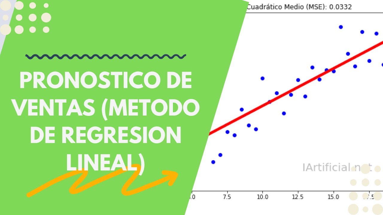
PRONOSTICOS DE VENTAS (Modelo Regresión Lineal)
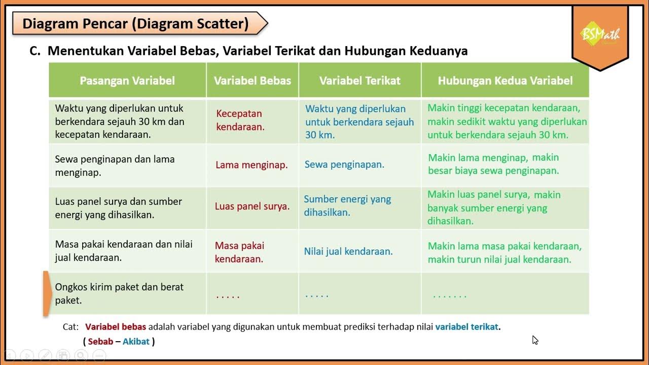
Menentukan Variabel Bebas dan Variabel Terikat - Matematika Wajib SMA Kelas XI Kurikulum Merdeka
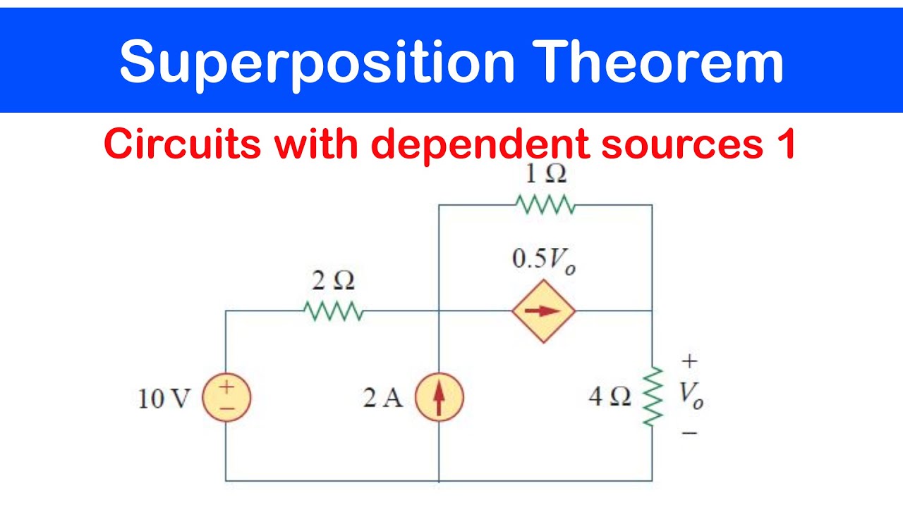
☑️19 - Superposition Theorem: Circuits with Dependent Sources 1
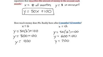
Real Life Linear Equations
7 Postulates of Quantum Mechanics
INDEPENDENT AND DEPENDENT VARIABLES || PRACTICAL RESEARCH 2
5.0 / 5 (0 votes)