Understanding the Discrete Fourier Transform and the FFT
Summary
TLDRThis MATLAB Tech Talk video, hosted by Brian, delves into the Discrete Fourier Transform (DFT) and its efficient computation through the Fast Fourier Transform (FFT) algorithm. It explains why DFT is essential for analyzing signals in the frequency domain, which isn't always apparent in the time domain. The video clarifies concepts like the amplitude spectrum, power spectrum, and power spectral density, while demonstrating the DFT's process with a graphical MATLAB app. It also addresses practical questions about interpreting FFT results, the difference between one-sided and two-sided FFTs, and the significance of bin width and frequency resolution in signal processing.
Takeaways
- 🔨 The script discusses the process of analyzing hardware vibrations using a shaker table and accelerometers, emphasizing the importance of understanding frequency components of the signal.
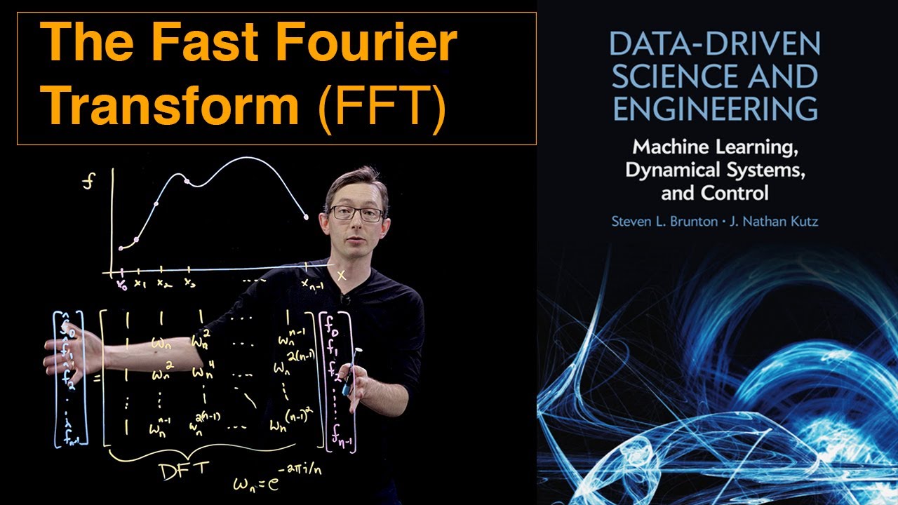
- 📈 The Discrete Fourier Transform (DFT) is introduced as a method to transform signals from the time or spatial domain into the frequency domain, making it easier to identify signal features.
- 🔍 The Fast Fourier Transform (FFT) algorithm is highlighted as an efficient way to compute the DFT, taking advantage of signal symmetries to reduce computational work.
- 🌐 The script explains the concept of frequency spectrum, amplitude spectrum, and power spectrum, which provide insights into the signal that time-domain analysis alone cannot.
- 🔄 The DFT equation is broken down to illustrate how the transformation works, involving multiplication of the time signal with sine and cosine signals of different frequencies.
- 📊 A MATLAB app demonstration is used to visually explain the DFT process, showing how it correlates the time signal with different frequencies to produce a frequency domain signal.
- 🔁 The script clarifies that the FFT returns both positive and negative frequencies, with the Nyquist frequency marking the boundary between them.
- 📉 The difference between one-sided and two-sided FFT is explained, with one-sided FFT focusing only on the positive frequencies for analysis.
- 📝 The importance of understanding the relationship between the variable k in the FFT and the actual frequency spectrum is discussed, including the concept of bin width.
- 🔧 The script provides practical advice on how to perform a one-sided FFT in MATLAB, including scaling considerations and the impact on frequency resolution.
- 🔬 The video concludes with a walkthrough of writing MATLAB code for a one-sided FFT, demonstrating the process from signal acquisition to frequency domain analysis.
Q & A
What is the purpose of using a shaker table in hardware testing?
-A shaker table is used to apply random vibrations to hardware in order to simulate real-world conditions and measure its response, ensuring the hardware can withstand such vibrations.
How does an accelerometer help in vibration analysis?
-Accelerometers are used to measure the response of the hardware to the vibrations applied by the shaker table, capturing the motion data which is then analyzed to understand the hardware's performance under vibration.
What is the main reason for transforming a signal from the time domain to the frequency domain?
-The transformation helps in identifying the frequency components of a signal, which may not be evident in the time domain, and provides insights into the signal's characteristics that are not apparent in the time or spatial domains.
What is the Discrete Fourier Transform (DFT) and why is it used?
-The DFT is a mathematical technique that transforms a signal from the time or spatial domain into the frequency domain, allowing for the analysis of the signal's frequency components.
How does the Fast Fourier Transform (FFT) algorithm improve upon the DFT?
-The FFT algorithm is an efficient way to compute the DFT by taking advantage of the symmetries in the matrix multiplication involved in the DFT, reducing the number of calculations required.
Why is the absolute value of the FFT often considered in signal processing applications?
-The absolute value of the FFT provides the magnitude of the frequency components, which indicates the presence and strength of specific frequencies in the signal without the need to consider their phase.
What is the difference between a one-sided and two-sided FFT?
-A two-sided FFT shows both positive and negative frequencies, while a one-sided FFT focuses only on the positive frequencies, which is often sufficient when dealing with real signals due to the mirrored nature of the spectrum.
How does the Nyquist frequency relate to the FFT?
-The Nyquist frequency is the highest frequency that can be accurately represented in the FFT and is based on the Nyquist sampling theorem, which states that the sampling rate must be at least twice the highest frequency of the signal.
What is meant by 'bin width' in the context of an FFT?
-Bin width refers to the frequency resolution of the FFT, which is the distance in frequency between adjacent points in the spectrum.
How does padding a signal with zeros affect the FFT?
-Padding a signal with zeros can improve the visualization of the FFT by reducing the bin width, but it does not increase the frequency resolution since no additional signal information is added.
Can you provide an example of how to calculate the one-sided FFT of a signal in MATLAB?
-Yes, to calculate a one-sided FFT in MATLAB, you would first take the FFT of the signal, then take the absolute value to get the magnitude, and finally, select only the first half of the spectrum, including the Nyquist frequency if present, and plot it against the corresponding frequencies.
Outlines

This section is available to paid users only. Please upgrade to access this part.
Upgrade NowMindmap

This section is available to paid users only. Please upgrade to access this part.
Upgrade NowKeywords

This section is available to paid users only. Please upgrade to access this part.
Upgrade NowHighlights

This section is available to paid users only. Please upgrade to access this part.
Upgrade NowTranscripts

This section is available to paid users only. Please upgrade to access this part.
Upgrade NowBrowse More Related Video

The Discrete Fourier Transform (DFT)
The Fast Fourier Transform (FFT)

Relation between Laplace transform, Fourier transform, z-transform, DTFT, DFT and FFT
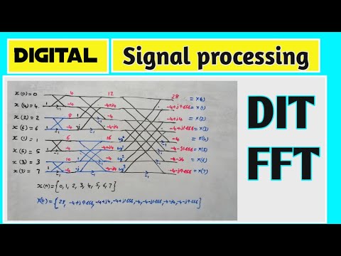
DIT FFT | 8 point | Butterfly diagram

DSP#44 problem on 8 point DFT using DIT FFT in digital signal processing || EC Academy

The Remarkable Story Behind The Most Important Algorithm Of All Time
5.0 / 5 (0 votes)