Calculating Power and the Probability of a Type II Error (A One-Tailed Example)
Summary
TLDRThis script discusses the calculation of power and the probability of a type II error, known as beta, using a one-sample Z test for a mean. It explains how to determine the rejection region for the null hypothesis that the population mean is 50, with a significance level of 0.09 and a known population standard deviation of 21. The script also explores how to calculate the probability of a type II error when the true mean is 43 or 40, illustrating the process with visual aids and standard normal distribution tables. It concludes by emphasizing the importance of correctly identifying the areas for power calculations in different scenarios.
Takeaways
- 🔍 The script discusses calculating power and the probability of a type II error (beta) in the context of a one-sample Z test on a mean.
- 🎯 The example involves a sample size of 36 from a normally distributed population with a known standard deviation (sigma = 21) and an unknown mean (mu).
- ⚖️ The null hypothesis is that the population mean is 50, and a one-sided alternative hypothesis is considered with a significance level (alpha) of 0.09.
- 📊 The Z test statistic is appropriate due to the normal distribution and known sigma, and the rejection region is determined based on the standard normal distribution.
- 📉 The rejection region is initially defined in terms of Z values and then translated into sample mean values (X bar) for power calculations.
- 📈 The script demonstrates how to find the critical value for rejecting the null hypothesis when the true mean is 43, resulting in a rejection region of X bar ≤ 45.31.
- 🛑 The probability of a type II error is calculated by determining the area under the sampling distribution of X bar to the right of the rejection region, given the true mean is 43.
- 🔎 The script shows how to standardize the sample mean to calculate the probability of a type II error and the power of the test.
- 📚 Power is defined as the probability of correctly rejecting a false null hypothesis, which is calculated as 1-beta.
- 🔄 The process is reiterated for a different true mean (40) to illustrate how power changes with different population means under the alternative hypothesis.
- 📋 The script emphasizes the importance of correctly identifying the areas under the standard normal curve for accurate power and type II error calculations.
Q & A
What is the significance level (alpha) used in the one-sample Z test example?
-The significance level (alpha) used in the one-sample Z test example is 0.09.
What is the population standard deviation (sigma) in the example?
-The population standard deviation (sigma) is known to be 21.
What is the null hypothesis being tested in the example?
-The null hypothesis being tested is that the population mean (mu) is 50.
What is the alternative hypothesis for the one-sample Z test?
-The alternative hypothesis is that the population mean (mu) is less than 50.
What is the Z value that corresponds to the alpha level of 0.09 in the standard normal distribution?
-The Z value with an area of 0.09 to the left is approximately -1.34.
What is the rejection region for the null hypothesis in terms of the sample mean (X bar)?
-The rejection region for the null hypothesis in terms of the sample mean (X bar) is less than or equal to 45.31.
What is the probability of committing a type I error in this scenario?
-The probability of committing a type I error, which is the probability of rejecting the null hypothesis when it is true, is 0.09.
If the true population mean is 43, what is the probability of a type II error?
-If the true population mean is 43, the probability of a type II error (beta) is approximately 0.255.
What is the power of the test when the true population mean is 43?
-The power of the test when the true population mean is 43 is 1 - beta, which is approximately 0.745.
If the true population mean is 40, what is the power of the test?
-If the true population mean is 40, the power of the test is the probability that the sample mean (X bar) is less than or equal to 45.31, which is approximately 0.935.
How is the power of a test defined in the context of hypothesis testing?
-The power of a test is defined as the probability of rejecting the null hypothesis when it is false, which is equivalent to 1 - beta.
Outlines

This section is available to paid users only. Please upgrade to access this part.
Upgrade NowMindmap

This section is available to paid users only. Please upgrade to access this part.
Upgrade NowKeywords

This section is available to paid users only. Please upgrade to access this part.
Upgrade NowHighlights

This section is available to paid users only. Please upgrade to access this part.
Upgrade NowTranscripts

This section is available to paid users only. Please upgrade to access this part.
Upgrade NowBrowse More Related Video
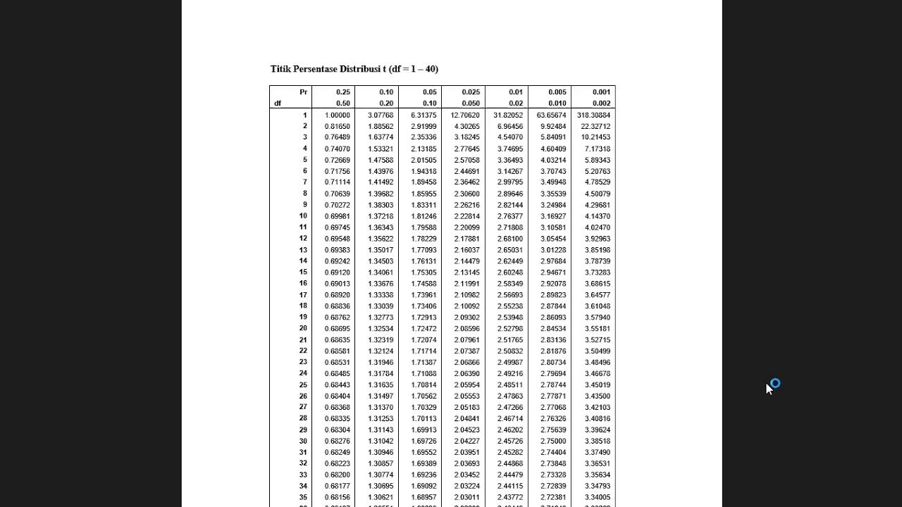
Uji beda mean 1 sampel dan T dependent
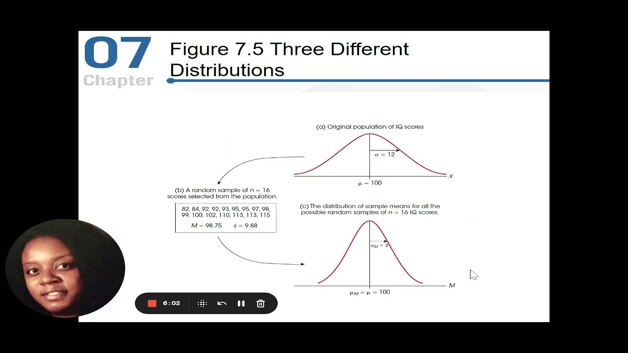
Chapter 7 Probability and Samples The Distribution of Sample Means
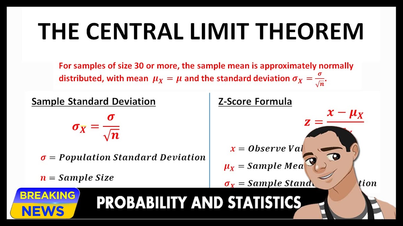
THE CENTRAL LIMIT THEOREM
Z-statistics vs. T-statistics | Inferential statistics | Probability and Statistics | Khan Academy
Confidence Interval for Mean with Example | Statistics Tutorial #10 | MarinStatsLectures

One-Sample T Test - Pertemuan 6
5.0 / 5 (0 votes)