Understanding Power Spectral Density and the Power Spectrum

Summary

The video explains how to interpret and scale a Fast Fourier Transform (FFT) to gain meaningful insights about a time domain signal. It covers converting an FFT into amplitude, power, and power spectral density representations. The choice of representation depends on the analysis goal and signal characteristics. Key factors are using a rectangular window, ensuring a stationary signal, and accounting for spectral leakage. With the right approach, the FFT can reveal a signal's dominant frequencies and power spectrum. However, broadband signals require looking at power spectral density. Overall, matching the FFT analysis technique to the signal and end goal enables gaining accurate, physically meaningful insights.

Takeaways

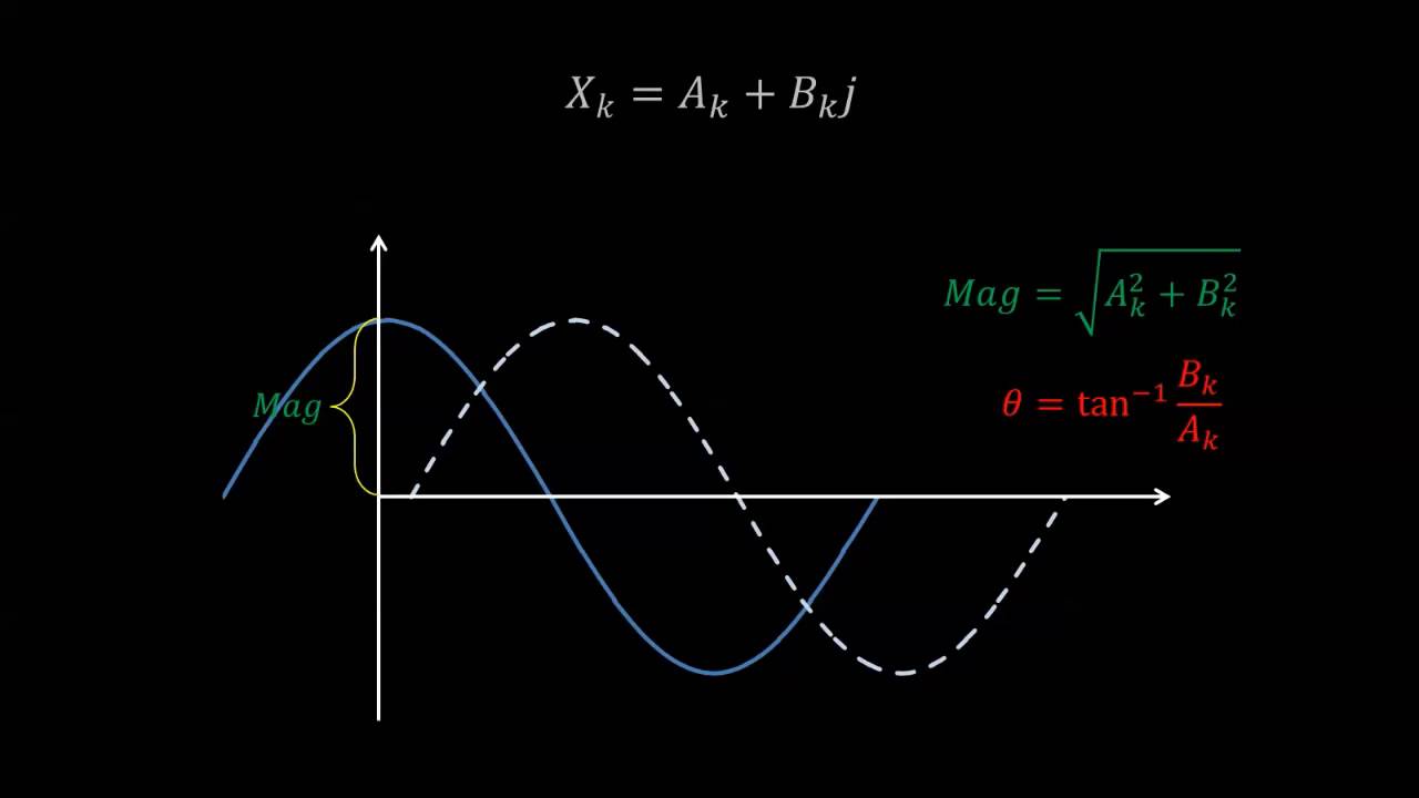
• 😀 The FFT transforms a time signal into a vector of complex numbers representing the signal's phase and magnitude at different frequencies.
• 👍 Scaling the FFT properly is key to understanding time domain signal properties from the frequency domain.
• 🤔 Choosing how to scale the FFT depends on your analysis goal - amplitude, power, power spectral density etc.
• 💡 Taking the absolute FFT value divided by N gives the amplitude. Squaring that result gives the power.
• ⚠️ Those equations only hold for rectangular windows on stationary, discrete spectra signals.
• 🔍 The power spectrum shows power of dominant sine waves. The power spectral density works better for broadband signals.
• 😕 Using the wrong FFT scaling leads to misleading results about time domain properties.
• 📈 Longer FFT windows reduce spectral leakage but limit frequency resolution.
• 🌄 The periodogram function handles windowing and scaling automatically.
• 💯 Understanding signal characteristics and analysis goals allows proper interpretation of FFT results.

Q & A

What is the purpose of doing spectral analysis?

The purpose is to understand quantitative properties of the signal in the frequency domain, such as the amplitude of sine waves at particular frequencies. The analysis method depends on your specific goal.

Why do we divide the FFT by N to get the amplitude?

Dividing by N gives us the average amplitude across the window. This works because of the mathematical derivation of the discrete Fourier transform and properties of sine waves.

When can we use the power spectrum equations for amplitude and power?

The equations are only valid when using a rectangular window, the signal is stationary within the window, and the signal has a discrete frequency spectrum.

How does window size affect the power spectrum?

A longer window reduces spectral leakage but also reduces frequency resolution. Windowing affects amplitude and power calculations.

What is spectral leakage and how can it be reduced?

Spectral leakage occurs when the signal period is not an integer multiple of the window length. It can be reduced by using a longer window or applying a non-rectangular window.

What is power spectral density and when should it be used?

Power spectral density normalizes the power spectrum. It should be used for signals with a continuous frequency spectrum rather than discrete spectral components.

How do you calculate the equivalent noise bandwidth?

The equation squares each window term, sums them, multiplies by the sample rate, and divides by the sum of window terms squared.

What does the power spectrum of a window represent?

It shows the attenuation of nearby frequencies that will blend together and contribute to each frequency sample.

Why can't power be accurately calculated when frequencies are too close?

Too close frequencies merge into a single peak that represents their combined power rather than individual power.

How can the periodogram function be used?

The periodogram function conveniently outputs the power spectrum or power spectral density and handles window normalization automatically.

Outlines

00:00

🔍 Understanding FFT Scaling for Signal Analysis

This segment introduces the concept of Fast Fourier Transform (FFT) scaling and its significance in signal analysis. It begins with a primer on FFT and its role in transforming a time-domain signal into a frequency-domain representation, consisting of complex numbers that embody both magnitude and phase of the signal's frequencies. The video addresses common confusions regarding the scaling of FFT outputs to derive meaningful information such as amplitude, power, and power spectral density. It emphasizes the importance of choosing the correct scaling approach based on the analytical goal, whether it be identifying frequency content or quantifying specific signal properties in terms of physical quantities. The explanation includes a practical demonstration using MATLAB, illustrating how to convert FFT results into one-sided amplitude and power spectra, thereby making the data relatable to physical aspects of the signal.

05:04

📐 Detailed Analysis of FFT Amplitude and Power Calculations

In this part, the video delves into the mathematical rationale behind FFT amplitude and power calculations, highlighting the importance of dividing by the total number of samples (N) for accurate measurement. It provides a step-by-step explanation of how FFT, fundamentally equivalent to the Discrete Fourier Transform (DFT), processes a signal to yield frequency domain coefficients. The discussion includes the mathematical derivation showing how the summation of sine and cosine products underpins the amplitude calculation, emphasizing the halving of amplitude due to its distribution across positive and negative frequencies. This section concludes with the method of obtaining one-sided power spectrum by squaring the amplitude and adjusting for the number of samples, demonstrating these concepts through MATLAB examples.

10:05

🚀 Mitigating Spectral Leakage and Understanding Windowing Effects

This segment explores the concept of spectral leakage and its mitigation through windowing techniques. It introduces the rectangular window as the simplest form of windowing, where signal samples within the window are unmodified, and explains how non-integer multiple frequencies of the window length can lead to spectral leakage. This leakage spreads signal energy across neighboring frequency bins, potentially distorting the analysis. The video discusses the use of non-rectangular windows, like the Hamming window, to attenuate signal edges and reduce leakage, albeit at the cost of resolution. It underscores the critical role of window choice in FFT analysis, affecting amplitude and power measurements, and demonstrates how MATLAB's periodogram function can accommodate different windows to produce accurate power spectra.

15:07

📊 Analyzing Power Spectral Density and Its Implications

The final part of the video focuses on power spectral density (PSD) and its significance in analyzing signals with continuous frequency spectra. It illustrates how discrete sine wave signals can be accurately analyzed for power using FFT, but when frequencies are too close or the signal is broadband, the analysis becomes more complex. The video explains how power from multiple frequencies contributes to the total in such cases, making PSD a more appropriate metric since it represents power per frequency band. It concludes with a practical MATLAB demonstration on calculating PSD by normalizing the power spectrum with the equivalent noise bandwidth, offering insights into how different types of signals require different analytical approaches to accurately reflect their physical properties.

20:09

📝 Conclusion: Choosing the Right Tool for Signal Analysis

The concluding segment emphasizes the importance of understanding the signal and the analytical objective when choosing between amplitude, power spectrum, and PSD for signal analysis. It reminds viewers that while mathematical tools can provide various views of the signal, connecting these analyses to physical properties requires careful consideration of the signal characteristics. The video encourages further exploration of FFT and DFT through additional resources, urging viewers to subscribe for more insightful content on signal processing and other topics. It positions the discussed concepts as foundational knowledge for effective signal analysis, underlining the utility of MATLAB in applying these principles.

Keywords

💡FFT (Fast Fourier Transform)

The FFT is a mathematical algorithm that computes the Discrete Fourier Transform (DFT) of a sequence, or its inverse, efficiently. In the context of the video, FFT is used to analyze the frequencies contained within a time-domain signal by converting it into a vector of complex numbers, representing the signal's magnitude and phase across different frequencies. The FFT is a fundamental tool in spectral analysis, allowing the detection of different frequency components within a signal, which is crucial for understanding its characteristics.

💡Magnitude

In the context of FFT analysis, magnitude refers to the size or strength of a frequency component within a signal, obtained by taking the absolute value of the FFT output. The video explains that analyzing the magnitude of the FFT, especially in a one-sided spectrum, helps identify the presence and relative strength of different frequencies in a time-domain signal. For example, the magnitude can reveal dominant frequencies or noise within a signal, providing insights into its behavior or composition.

💡Phase

Phase in the context of FFT represents the angle of the complex numbers resulting from the FFT, indicating the shift or displacement of the sinusoidal components of the signal relative to a reference point. The video mentions that in many practical applications, the phase information might be disregarded when only the magnitude of the frequencies is of interest, simplifying the analysis to focus on the strength of the frequency components.

💡One-sided Spectrum

A one-sided spectrum displays only the positive half of the frequency spectrum obtained from the FFT, which is sufficient for real-valued time-domain signals since the negative frequencies mirror the positive ones. The video highlights this concept by explaining that in many cases, focusing on the one-sided spectrum simplifies the analysis without losing meaningful information, as the negative side offers no additional insight for such signals.

💡Amplitude

Amplitude in the context of FFT analysis refers to the actual height or strength of a sinusoidal component within a signal, measured from its equilibrium point. The video elaborates on how to convert the FFT output into meaningful amplitude information by scaling the absolute values of the FFT by the number of samples, and then adjusting for a one-sided spectrum. This process allows the determination of the physical amplitudes of sinusoidal components within the original time-domain signal.

💡Power Spectrum

The power spectrum is a representation of the signal's power content distributed over the frequency domain. The video describes how to derive the power spectrum from the FFT by squaring its magnitude (to get power) and scaling appropriately. The power spectrum is particularly useful for analyzing the energy distribution across different frequencies within a signal, providing insights into its power characteristics at specific frequencies.

💡Spectral Leakage

Spectral leakage occurs when the discrete sampling of a signal causes the spread of signal energy across adjacent frequencies, particularly when the signal's frequency components do not align perfectly with the FFT bin frequencies. The video discusses spectral leakage in the context of windowing, explaining how it can distort the true frequency content of a signal and how applying different window functions can mitigate its effects.

💡Windowing

Windowing is a technique used in FFT analysis to manage the effects of analyzing a finite segment of a signal, often by applying a specific function to taper the signal at its boundaries. The video explains that while a rectangular window (which leaves the signal unmodified within the window) is straightforward, other window types like Hamming or Blackman can reduce spectral leakage by attenuating the signal edges, albeit at the cost of resolution.

💡Stationarity

A stationary signal is one whose statistical properties, such as mean and variance, do not change over time. The video emphasizes the importance of stationarity in FFT analysis, as non-stationary signals can lead to misleading average power or amplitude readings due to fluctuations within the windowed segment of the signal.

💡Power Spectral Density (PSD)

Power Spectral Density is a measure of a signal's power content per unit frequency, providing a detailed view of how power is distributed across frequencies. The video explains how to obtain PSD from the FFT by normalizing the power spectrum with respect to the frequency resolution, making it a valuable tool for analyzing signals with continuous spectra or for comparing power distribution across different frequency bands.

Highlights

Clarification on scaling an FFT for understanding time domain signal properties.

Differentiation between FFT amplitude, power, and power spectral density representations.

Discussion on the relevance of selecting specific FFT representations based on analysis goals.

Explanation of how to derive amplitude from an FFT.

Method to obtain amplitude of a sine wave from the FFT by dividing by total number of samples.

Demonstration of amplitude extraction from FFT using MATLAB.

Derivation of FFT amplitude scaling factor based on discrete Fourier transform.

Explanation of obtaining power from a signal's FFT.

Introduction of the concept of a one-sided power spectrum.

Illustration of converting FFT to one-sided power spectrum in MATLAB.

Discussion on the importance of using a rectangular window for accurate FFT results.

Explanation of spectral leakage and its mitigation techniques.

Requirement of signal stationarity for valid FFT analysis.

Impact of discrete versus continuous frequency spectra on FFT analysis.

Derivation and application of power spectral density from FFT.

Conclusion emphasizing the necessity of understanding signal characteristics for appropriate FFT analysis.

Transcripts

In this video, we're going to look

at how to get meaningful information from a fast Fourier

transform, from an FFT.

And I want to clear up what I see

is a lot of confusion on how to scale an FFT in a way that

provides an understanding of the properties of the time domain

signal.

Specifically, I want to cover how

we go from an FFT to amplitude and to power and to power

spectral density.

And I want to talk about why we may choose

one representation over another and the scenarios

in which they are valid.

I think this will be useful.

So I hope you stick around for it.

I'm Brian, and welcome to a MATLAB Tech Talk.

If you don't know what an FFT is,

then I recommend watching my video on it,

that I've linked to below.

But for right now, all that you really need to know

is that when you take an FFT of a signal,

it returns a vector of complex numbers.

And here, I'm just plotting the real and imaginary parts

of an FFT for time signal xn.

And these numbers represent the phase

and the magnitude of the frequencies

that exist within x sub n.

And in that video, we covered how, in some cases,

we aren't concerned with phase.

So we just look at the magnitude by taking

the absolute value of the FFT.

And then when dealing with real time signals,

the magnitude of the FFT is duplicated between the positive

and the negative frequencies.

And since the information is the exact same,

we can choose to only look at the positive frequencies,

a so-called one-sided FFT.

And this is where we left that video, with a one-sided plot

of magnitude, versus frequency.

Now, how can we use this information

to understand something about the time signal?

And when it comes to spectral analysis,

the question you have to start with is, why are you doing it?

What are you hoping to learn by analyzing a signal

in the frequency domain?

And the reason that this is an important question

is because the tool that you use to do your spectral analysis

depends on your goal.

And in the case of this video, how you manipulate

the FFT depends on your goal.

For example, if all you want to know

is where frequency content exists

in the signal relative to each other,

then this magnitude plot is sufficient.

I mean, I can tell that there is a strong frequency

component at 110 hertz, and there

is a weaker, but still obvious component at 100 hertz.

And this level of analysis might be

good for figuring out if there's a 60-hertz noise in a signal

or maybe, what the natural frequency is

of a structure that's vibrating.

So it's pretty cool that you can get that information

from the magnitude.

But the downside of this plot is that this value on the y-axis

isn't a quantity that relates to some physical property

of the time signal.

So what if you do want to know something

quantitative about the signal?

Say you want to know the amplitude of a sine wave

at a particular frequency.

Well, I'm going to spoil it for you.

This is how you do it.

You take the absolute value of the FFT

and then divide by capital N, which

is the total number of samples in the signal.

This produces amplitude, but it's

split, with half of the amplitude being captured

in the positive frequencies and the other half

in the negative frequencies.

And so if we just want to look at a one-sided spectrum,

we ignore the negative frequencies and double

the values for every positive frequency

except for the DC term, which is 0 hertz, and the Nyquist

frequency.

And we can go over to MATLAB and see that this works.

It actually returns the amplitude of a sine wave.

I have a time signal with two sine waves

with amplitudes 1 and 4.

And then I take the absolute value of the FFT,

divide by the number of samples, and then look at just one side

and double it, except for the DC and Nyquist.

And when I plot this spectrum, the y-axis

now shows amplitudes of 1 and 4, so perfect.

But the question might be, is why are we dividing by N?

I mean, why does this work, in the first place?

Well, let's quickly walk through an explanation.

OK, so the FFT is mathematically equivalent

to the discrete Fourier transform, which

says that we start with a time signal xn,

multiply it by a correlating signal, which

is this exponential here, and then sum over

all of the samples.

And this produces the frequency domain coefficients xk.

Also, e raised to an imaginary number

is just a function of cosine and sine.

All right, so now let's say that the time signal is just

a sine wave with amplitude A. And it

doesn't matter what frequency it's at, so I'm just

going to put a dot in here.

And if we plug this into the DFT,

we get that xk is equal to the amplitude A times the summation

over all of the samples of sine times

cosine minus i times sine squared.

And sine times cosine produces another sinusoid.

And so the summation over one period is 0.

It cancels each other out.

So no matter how long the signal is,

the summation will always be close to 0l.

And therefore, this first component

doesn't contribute much to the summation.

Sine squared, on the other hand, looks like this,

like a sinusoid that goes between 0 and 1.

And since this is discrete, we're sampling it n times.

Now, the more samples we have, the larger this summation

will be.

However, if we add up all of the samples

and then divide by the number of samples,

this will give us the average height

of the sine squared function, right?

I mean, if you add up 10 numbers and divide by 10,

you get the average value.

Well, the average value for sine squared is 1/2.

So if we go back to the above equation,

we can divide xk by N. And now, this whole summation

is 0 for the first component still.

But it's 1/2 i for the second component,

since it's just the average height of sine squared.

Now we're taking the absolute value

of x of k, which gives us the magnitude of the FFT.

And that is equal to 1/2 the amplitude.

And again, the reason that it's in half here

is because the amplitude is split

between the positive and negative frequencies.

But if we're just looking at a one-sided FFT,

then we're multiplying this by 2.

And we're left with amplitude.

Now, I just want to note that if our original time signal had

a phase shift to it, this all still works out mathematically.

I just did a 0 phase sinusoid to make it easier to follow.

But I think overall, this is pretty cool,

that we can find the amplitude of a sinusoid

simply by taking the FFT and scaling it.

All right, so that's amplitude.

But what if we want to know power

at a particular frequency?

Well, the average power of a sinusoid

is just its amplitude squared over 2.

And since we know that the absolute value

of the FFT divided by N gives us the amplitude over 2,

then the easiest thing we can do is just square that value.

And this is the two-sided power spectrum,

since the power is split between negative and positive

frequencies.

So to get the one-sided power spectrum, we multiply it by 2.

And this is how we go from the FFT

to the one-sided power spectrum.

So let's go back over to MATLAB and see

how we can implement this.

This, by the way, is the same script as before.

So we're working with the same two-sine wave signal.

And I'm just going to scroll down past Amplitude

and get to the Power section.

So here, I'm taking the absolute value of the FFT,

then squaring it and dividing by N squared.

And then to get a one-sided power spectrum,

we ignore the negative frequencies

and double the positive frequencies,

again, except for DC and Nyquist.

Now, the plot looks like this, with powers of 1/2 and 8,

which correspond to the amplitudes 1 and 4,

respectively.

So it all works out nicely.

But often, we like to look at power in decibels.

So let me do that here real quick with the Pow

to dB function and then rerun this script.

And this is the one-sided power spectrum that I created,

and it took several lines of code.

But you can type all of this out each time you want

to get to the power spectrum.

Or you can just get the exact same result

with the periodogram function.

And there's many different ways to create a periodogram.

But here, I'm running it with a rectangular window in FFT,

which is the length of the entire signal,

and then setting it to return the power spectrum instead

of power density.

These are the parameters that exactly

copy what we just coded above.

And you're going to have to take my word for it here,

but these two plots are identical.

So there we go, right?

To get one-sided amplitude, we take 2 times the absolute value

of the FFT and divide by N. And to get power,

we take 2 times the absolute value of the FFT

squared and divide by N squared.

That's pretty easy, right?

Well, kind of.

We have to be really careful here

because these results are only true if there are

three very important things.

One is that we're using a rectangular window and not

some other window, like Hamming or Blackman.

Two, the time signal is stationary.

And three, we're dealing with time signals that

produce discrete frequency power spectra and not

a continuous spectrum.

So let me go through each of these

and explain why they're important for these equations

to hold.

And we're going to start with the rectangular window.

When we take the FFT of a time signal,

it necessarily must be finite.

There is a start time and an end time.

And therefore, we're really only looking

at a small subset of the total possible infinite signal.

And from this subset, we're trying to understand the signal

properties.

And this subset of data is called a window,

since we're only looking at a portion,

and the rest is obscured from view.

Now, the window could be long, or it could be short.

Or we could look at a different part of the signal altogether.

But no matter what, we're always just looking at a subset.

Now, what I've drawn here is a rectangular window.

And this means that each sample in the window is unmodified.

That is, we multiply everything inside the window by 1

and then 0 for everything outside of the window.

And this makes sense, right?

I mean, why would you want to change your signal if you're

trying to find out the properties of that signal?

Well, one reason is for spectral leakage.

And one way that spectral leakage occurs

is when the period of a time signal frequency

is not in integer multiple of the window length.

In these cases, cutting a period short

like this spreads that signal energy out

into neighboring frequency bins, since that summation

that we talked about earlier doesn't get

fully canceled out by having a complete period.

And one way to mitigate this is to just use a longer time

series because that leftover period gets

averaged across a longer time span.

But if that isn't possible, then another way

is to just apply a non-rectangular window

to your data, something like a hamming window, that

attenuates the signal near the edges

and reduces the effect of that partial period.

Now, this reduces the spectral leakage,

but it also comes at a cost of lower resolution.

And I'm not going to cover different windows much

in this video, I just want you to be aware

that you might not always be dealing

with a rectangular window.

And as you might expect, if you attenuate

the signal near the edges, you are, of course,

affecting the average amplitude and the average power

within that window.

Therefore, for the equations that we

derived for amplitude and power are only

valid for rectangular windows.

And there are ways to account for the effects of the window

when looking at power, which I'm not

going to cover in this video.

But if we go back to MATLAB and the periodogram function,

we can see that it does handle the effects of the window.

Because both hamming and rectangular windows

produce the correct power for the 110-hertz frequency

that I'm showing here.

All right, for the second requirement,

the time series must be stationary.

And this just means that the signal

from a statistical standpoint doesn't change over time.

The mean and the variance of the signal

are the same regardless of where you look.

And here's a way to understand why it's a requirement.

Remember back when we were deriving the amplitude,

we divided by N because we were looking

for an average amplitude?

And we had an assumption that the amplitude

is relatively constant across the window, right?

I mean, take, for example, this signal.

It's a single frequency, but the power

is changing throughout the window.

If we calculate the power for this frequency,

it will give us an average across the window.

But it won't provide any indication

that the power is changing.

Now, a worst-case scenario of this

is if there is a very short-term, high-powered event

that is just averaged across a long window,

potentially causing it to be lost in the noise.

All right, so we know that we want a rectangular window.

And we want the signal within that window to be stationary.

Now, for the third requirement, we

need the signal to have discrete spectra.

And why this is required is really important.

To explain why, let's go back over to MATLAB.

Here, I have a time signal with two sine waves,

one at 100 hertz and one at 110 hertz.

And then I'm taking the FFT and then scaling it

for the power spectrum.

Now, what I'm plotting here is the true power

for the two sine waves.

And that's the red and yellow stems.

And I'm also plotting the power spectrum

for the signal, which is the blue curve.

And notice how these peaks for the blue curve

aren't perfectly sharp, but they're

spread out a little bit.

And this comes from spectral leakage

that occurs because we're using that finite window.

But the important thing is that the peak of the power spectrum

is at 8.

So even with this spread, we're getting an accurate measurement

of the power at these frequencies.

Now, let me hide the code here so that we

can focus on this graph.

And watch as I move the frequency of the second sine

wave closer to the first.

At some point, their spectra start

to interfere with each other.

And then when they're too close, they merge into a single peak.

Now, the value of the y-axis isn't reporting an accurate

power at that frequency.

In fact, we can't say much of anything

about the power of each individual sinusoid.

What's being reported is some combination

of the two frequencies, that are just too close to each other

to separate out.

Now, this is just two discrete sine waves.

But imagine the case of broadband signals,

where the frequency spectrum is continuous.

In this plot, I'm showing 50 sinusoids

between 100 and 100.5 hertz.

And each of them contribute a very small amount of power.

But if I zoom out, we can see that the power spectrum

for the time signal is much higher because they all

contribute a little bit to that total.

So hopefully, you can see that this peak doesn't represent

a power at a particular frequency,

but the power of all of the frequencies

that contribute to it.

So in some way, it represents power density.

This area is much more dense than these areas are,

and we can tell that from the peak.

And we can normalize this plot by dividing it

by some frequency bandwidth, specifically,

the equivalent noise bandwidth, which is, in some way,

the width of the frequencies that

contribute to a particular sample in the power spectrum.

And it is a function of the window itself.

A finite length window will necessarily

blend the power of nearby frequencies

together, like we saw.

And we can see how this blending occurs

by looking at the power spectrum of the window itself.

For a rectangular window of length 128 and sampled

at 1000 hertz, this is its power spectrum.

And I've shifted the negative frequencies

to be over on the left, so that we get a better sense of what

this curve looks like. l And notice

that the window has a maximum power of 1, right at 0 hertz.

So the way that we can interpret this

is that this window will pass through the power

for the frequency that is being sampled unmodified.

It's multiplying it by 1.

So in this way, we can accurately get the power

from a single sine wave.

However, along with that value, this window

will also add in the power at all of these other delta

frequencies attenuated by the amount given by the curve.

The longer the window, the steeper

the curve, which means that a longer window will have fewer

contributions from nearby frequencies

than a shorter window does.

All right, so each sample in the spectrum

is the summation of the attenuated power from all

of these nearby frequencies.

So we might think that the bandwidth we're interested in

is however far out this tail goes,

since all of those frequencies are included in some way.

But as we can see these, far-away frequencies

don't contribute very much.

We really only want to consider the frequencies that

have the most impact.

And the way we find that is to approximate this curve, using

a rectangle with height equal to the peak

and whose area is equal to the total power.

So the area under the blue curve is

equal to the area under the red rectangle.

And the width of this rectangle is the equivalent noise

bandwidth.

And under this assumption, we can

say that this is the range of frequencies that contribute

to each sample in the spectrum.

And so to get power spectral density,

we divide the power spectrum by the equivalent noise bandwidth.

And we know power spectrum.

It's the absolute value of the FFT

squared divided by N squared.

And this is the equation for the equivalent noise bandwidth

for an arbitrary window.

And I'll leave a link below to a derivation for it.

But the way that we read this is that we

square each of the terms in the window,

and then sum them all up and multiply that by the sample

rate, and then divide by the sum of the window

terms, which is then squared.

And so for a rectangular window, each of the N terms

have a value of 1.

And so this just becomes fs times N over N squared,

or fs divided by N. And now, when we divide the power

spectrum by this, the Ns cancel out,

and we're left with 1 over fs times N

times the absolute value of the FFT squared.

And this is the scaling for power spectral density

using a rectangular window.

And for the last time in this video,

let's go back to the MATLAB script and see it in action.

And you know what's going on at this point, right?

We're just taking the absolute value of the FFT,

squaring it, and dividing by fs times N. And voila, the power

spectral density.

And instead of typing all of this out again,

we can use the periodogram function to generate the PSD.

And the nice thing about this function

is that it's really easy to change the output to power

or to change the window and see the results really quickly.

Now, if you want to play around with this script a little bit,

I've left a link to it below.

But I hope that this whole thing has cleared up some confusion

about the FFT and power.

And the thing to remember is that if your signal is made up

of a few dominant sine waves, then

you can look at the power spectrum

to get the power in those frequencies.

However, if there are broadband signals,

then it probably makes more sense to look at the PSD

instead, since that returns the power per frequency band.

And mathematically, you can take the PSD of a single sine wave

or the power spectrum of wide band signals,

and you're going to get a plot.

But the trouble comes when you try to tie those plots back

to some physical property in the time domain.

Because they just won't make much sense.

And this is why you have to know what you're

trying to accomplish and what kind of signal

you're looking at, in order to choose the correct tool.

All right, so that's where I'm going to leave this video.

Don't forget to subscribe to this channel

so you don't miss any future videos.

Also, you can find all of the Tech Talk videos

across many different topics nicely organized

at mathworks.com.

And if you liked this video, then you

might be interested to learn about the Fast Fourier

Transform in our video on the FFT and the DFT.

All right, thanks for watching, and I'll see you next time.