Solving Delay Differential Equations With Julia | David Widmann | JuliaCon 2019
Summary
TLDRThe speaker, a PhD student at Uppsala University, discusses their research on solving delayed differential equations (DDEs) using Julia's differential equations package ecosystem. They explain the concept of DDEs, which extend ordinary differential equations by incorporating past values of the state, and highlight the challenges in solving them due to potential discontinuities and richer dynamical structures. The presentation outlines the process of formulating DDEs in Julia, leveraging existing solvers for ordinary differential equations, and the innovative approaches taken to handle discontinuities and state-dependent delays. The speaker also shares their experience with the Julia package, their contributions to it, and the successful simulation of complex models, emphasizing the potential for further enhancements like Anderson acceleration and the development of stochastic DDE solvers.
Takeaways
- 🎓 The speaker is a PhD student at Uppsala University researching uncertainty in deep learning but is presenting on solving delayed differential equations (DDEs).
- 🔍 The speaker's initial work on DDEs began during their master's project at Technical University in Munich, involving comparing two models formulated as DDEs.
- 💡 The motivation for contributing to the Julia differential equations package ecosystem stemmed from the need to simulate models reliably for parameter estimation.
- 🧩 DDEs extend ordinary differential equations (ODEs) by allowing the derivative to depend on past values of the state, which is crucial for modeling certain biological phenomena.
- 📉 The speaker faced issues with simulating DDEs, including negative concentrations and unreliable simulations, prompting the opening of issues and pull requests in the Julia ecosystem.
- 🛠 The 'delayed' package in Julia was improved by the speaker to address the inability to solve their specific problem, incorporating functionality from the existing ordinary differential equation solvers.
- 🔬 DDEs can exhibit richer dynamical structures, such as chaotic behavior, even in scalar cases, which is not possible with ODEs unless there are at least three components.
- 📝 The formulation of DDEs in Julia's 'delayed' package closely mirrors that of ODEs, but with the critical addition of dependence on past state values.
- 🔄 The 'delayed' package uses a method of steps approach, leveraging the existing ecosystem of ODE solvers in Julia to iteratively solve DDEs by breaking them down into a sequence of ODEs.
- 🚧 Challenges in solving DDEs include handling discontinuities and ensuring the solution's smoothness, which the 'delayed' package addresses by tracking discontinuities and using fixed point iteration.
- 🔭 Future work for the 'delayed' package includes implementing Anderson acceleration to speed up fixed point iterations and conducting more extensive benchmarking.
Q & A
What is the main research topic of the speaker at Uppsala University?
-The speaker is a PhD student at Uppsala University, and their main research topic is about uncertainty in deep learning.
What was the initial problem the speaker faced during their master's project?
-The speaker faced issues with simulating trajectories for two different models formulated as delay differential equations, which led to negative concentrations and unreliable simulations.
Why did the speaker choose to work with Julia instead of MATLAB for solving differential equations?
-The speaker chose Julia because they had heard about its great ecosystem for solving differential equations and encountered issues with MATLAB that they did not attempt to fix.
What is a delay differential equation and how does it differ from an ordinary differential equation?
-A delay differential equation is an equation in which the derivative can depend on past values of the state, unlike ordinary differential equations where the derivative only depends on the current time and state.
Can you provide an example of a delay differential equation?
-An example given in the script is Hutchinson's equation, which models population growth with a delay, taking into account resources available at a previous time point.
What are some challenges in solving delay differential equations compared to ordinary differential equations?
-Challenges include the need for a history function instead of just an initial condition, the potential for discontinuities in the solution, and a richer dynamical structure that can exhibit chaotic behavior even in scalar cases.
How does the DelayDiffEq package in Julia handle the solution of delay differential equations?
-The DelayDiffEq package uses a method of steps approach, leveraging the existing ecosystem of ordinary differential equation solvers in Julia by setting up a dummy solver and wrapping the history function to evaluate the solution at any time point.
What is the significance of tracking discontinuities in delay differential equation solvers?
-Tracking discontinuities ensures the correct level of smoothness in the solution and helps solvers hit discontinuities accurately without stepping over them, which is crucial for the accuracy and efficiency of the solution.
How did the speaker and their team improve the efficiency of solving state-dependent delay differential equations?
-They improved efficiency by implementing fixed point iteration for state-dependent delays and updating the method for tracking discontinuities, which allowed for better use of stiff solvers from ordinary differential equations.
What are some future improvements planned for the DelayDiffEq package?
-Future improvements include the potential use of Anderson acceleration to speed up fixed point iterations and more extensive benchmarking to further refine the solver's performance.
Can the speaker provide an example of how to specify a delay differential equation problem in Julia?
-Yes, the speaker can provide an example, which involves specifying a history function, initial values, and the timespan for integration, similar to how ordinary differential equations are specified in Julia.
How does the speaker plan to demonstrate the solution of a delay differential equation in Julia?
-The speaker mentioned working on a special branch to implement Anderson acceleration and is willing to live code the problem after precompiling, to show how the problem is solved in Julia.
Outlines
📚 Introduction to Uncertainty in Deep Learning and Delay Differential Equations
The speaker introduces themselves as a PhD student at Uppsala University, focusing on uncertainty in deep learning. They delve into their background in mathematics and medicine from Technical University in Munich and recount their initial encounter with delay differential equations (DDEs) during their master's project in mathematical biology. The speaker describes their experience with simulating models formulated as DDEs and the challenges they faced, which led them to contribute to the Julia differential equations package ecosystem. They set the stage for the presentation by expressing the need for a reliable simulation tool for parameter estimation and comparison of models, hinting at the improvements they made to the DDE package in Julia.
🔍 Exploring Delay Differential Equations and Their Characteristics
This paragraph delves into the nature of delay differential equations, contrasting them with ordinary differential equations (ODEs). The speaker explains that DDEs allow the derivative of a function to depend on past values, which is particularly useful in modeling real-world phenomena where changes do not occur instantaneously, such as in epidemiology or population growth models. The paragraph introduces the concept of constant and time-dependent delays, as well as neutral delay differential equations. The speaker also discusses the challenges in solving DDEs, such as the need for a history function instead of just an initial condition and the potential for discontinuities in the solution. They provide an example of a logistic growth model and its delayed counterpart, highlighting the complexities introduced by the delay.
📉 Challenges and Dynamics of Solving Delay Differential Equations
The speaker discusses the differences between solving ordinary differential equations and delay differential equations, emphasizing the need for a history function and the potential for discontinuities in the solution. They highlight that even if the initial function and model are smooth, discontinuities can arise, which propagate through time, affecting the solution's dynamics. The speaker also touches on the richer dynamical structure of DDEs, which can exhibit chaotic behavior even in scalar cases, unlike ODEs. They provide a visual example of a simple DDE with constant delays and its resulting discontinuities over time. The paragraph concludes with a brief mention of how DDEs can be formulated in Julia, drawing parallels to the formulation of ODEs.
🤖 Leveraging Julia's Ecosystem for Solving DDEs
The speaker outlines the approach to solving delay differential equations using Julia's ecosystem, which includes a variety of algorithms for ordinary differential equations. They describe the method of steps, which involves iteratively solving a sequence of ODEs, and how this can be applied to DDEs with constant delays. The speaker also explains how the existing functionality in Julia's ordinary differential equation (ODE) package can be utilized for solving DDEs, by setting up a dummy solver and using the initial function provided by the user. They highlight the importance of updating the solution and solver at each time step to maintain an accurate history function for the DDE.
🛠 Addressing Discontinuities and Efficiency in DDE Solvers
This paragraph addresses the challenges of handling discontinuities and ensuring efficiency in delay differential equation solvers. The speaker explains that ordinary differential equation algorithms assume a smooth solution, but discontinuities can occur, which requires special handling. They discuss the use of fixed point iteration for small delays and the tracking of discontinuities up to the order of the solver. The speaker also mentions the recent improvements made to the DDE solver in Julia, which allows for more efficient handling of state-dependent delays. They conclude with an example of how using stiff solvers from the ODE package can significantly improve the simulation of a DDE model.
🚀 Future Enhancements and Contributions to the DDE Solver
The speaker wraps up the presentation by discussing future enhancements to the delay differential equation solver. They mention the potential use of Anderson acceleration to speed up fixed point iterations and the need for more extensive benchmarking. The speaker acknowledges the contributions of others to the development of the DDE solver and expresses gratitude for the collaborative efforts. They also hint at the possibility of live coding an example and discuss the potential for stochastic delay differential equation solvers, indicating that this is an area of interest for future development.
🔗 Closing Remarks and Future Collaborations
In the final paragraph, the speaker expresses their excitement about meeting in person after years of online interactions and hints at the potential for future collaborations, especially in the area of neural differential equations. They also touch on the topic of stochastic delay differential equations and the possibility of contributing to their development. The speaker leaves the audience with a sense of anticipation for future advancements in the field and the potential for continued collaboration.
Mindmap
Keywords
💡Uppsala University
💡Deep Learning
💡Delayed Differential Equations
💡Julia
💡Ordinary Differential Equations (ODEs)
💡Pharmacodynamics
💡Stiff Solvers
💡Parameter Estimation
💡Anderson Acceleration
💡Fixed Point Iteration
💡Stochastic Delay Differential Equations
Highlights
Introduction of the speaker as a PhD student at Uppsala University researching uncertainty in deep learning.
The speaker's work on a package for solving delayed differential equations during their master's studies at Technical University in Munich.
Initial issues encountered with simulating trajectories for models formulated as delay differential equations.
Contribution to the Julia differential equations package ecosystem by opening issues and pull requests.
Explanation of the difference between ordinary differential equations and delay differential equations.
Characteristics of delay differential equations, including their dependence on past values of the state.
Challenges in solving delay differential equations compared to ordinary differential equations.
The need for a history function or initial function for delay differential equations, as opposed to just an initial condition.
Potential discontinuities in delay differential equations due to difficulties in enforcing equal left and right derivatives at the initial time point.
Rich dynamical structures of delay differential equations, including the possibility of chaotic behavior even in scalar cases.
Formulation of delay differential equations in Julia, leveraging the existing ecosystem for ordinary differential equations.
Use of a dummy solver to handle the history function and previous states in delay differential equations.
Addressing discontinuities in delay differential equations by tracking them up to the order of the solver.
Innovations in handling state-dependent delays by performing fixed point iteration and using extrapolation.
Efficient simulation of models with delay differential equations using stiff solvers from the ordinary differential equation package.
Future plans for the delay differential equation package, including the potential use of Anderson acceleration and more extensive benchmarking.
Invitation for the speaker to contribute to the development of stochastic delay differential equation solvers.
Transcripts
thank you very much for this
introduction and hi everyone I guess you
can hear me it feels like like
everything is fine and setup yeah as you
already heard I'm at the Uppsala
University at the moment I'm a PhD
student there doing research about
uncertainty a very deep learning and
that might sound a bit strange since the
topic of my my presentation today is
solving delayed differential equations
and so I think I have to explain that a
bit more I mainly worked on this package
or started to work at least at the end
of my master studies at the Technical
University in Munich so before I went
into Salah and started my PhD there I
had been studying mathematics and
medicine in Munich and so at the end of
my master studies when I had to pick a
topic for my Master's project and then I
picked something a bit more applied from
mathematical biology and basically the
details are not interesting here now but
it was about comparing two different
models and these models were formulated
as delay differential equations so the
first thing when I started my work on
this most project the first thing I did
was take some parameter guesses that
some other people had estimated for one
of those two models and tried to
simulate a trajectory and that's what
happened basically so that's the
earliest github issue I think I could
find that I opened at the Julia
differential equations package ecosystem
and here I already fine-tuned that a lot
so I try to incorporate the fact that
this some concentration that it cannot
be negative and try to adjust the step
sizes and tolerance is a bit but as you
can see that's not something that you
would like to to get in your simulation
and and I mean I I also wanted to do
parameter estimation and then with both
models I want you to compare them I want
you to run many of these simulations and
they they should work reliably and so it
felt like yeah there's something missing
here and yeah that's why I opened this
first issue and then I actually also
tried to use MATLAB even though I wanted
to use julia also because i had heard
about this great ecosystem for solving
the differential equations in julia and
and also there I had issues so I
immediately went back to you - Julia I
didn't try to fix the issues in MATLAB
and instead I started to open issues and
then also pull requests after some time
and so I started to contribute - yeah
the delay differential equation package
which was existing at that time but
apparently could not solve my problem
and so now today in this talk I want to
to explain basically I yeah what you can
do with this package right now on how I
was able to solve these issues and yeah
but first before I do that I I quickly
explain able to delay differential
equations actually are and some of the
characteristics which makes it a bit
more difficult maybe to to
solve than ordinary differential
equations so yeah let's start with
ordinary differential equations which I
guess more people are familiar with or
have even used the player Julia package
simulating them I mean for example in
the keynote talk today we heard that
they're used in pharmaco dynamics and
also in many other scientific areas
differential equation models and
especially also ordinary differential
equation models are used I think there
are two nice things that you can
incorporate in this function f some
prior assumptions some prior knowledge
but still you have don't have to specify
the dynamics of X explicitly and so but
there is some more or less implicit
assumption I mean it's quite explicit
from from this from this formulation but
that this the derivative at the time
point can only depend on the current
time point and the state at the current
time but for example in biology many
changes do not occur instantaneously
for example thinking about a pity on me
epidemiology then some yeah
disease is there you have an incubation
period or also if think about
reproduction and then birth then yeah it
takes some time for human nine months
usually until yeah you're actually born
and it has an effect on the birth rate
so yeah for animals for example you
could think that the birth rate depends
on how many resources were available at
the time point for example nine months
earlier and that's it cannot be captured
by this form of differential equations
so delay differential equations then are
basically ordinary differential
patience in which this derivative can
also depend on past values of the state
and so very simple form of delay
differential equations you can see here
there you have a dependence on the state
at time t minus tau and now this tau
here is a constant so that's called a
constant delay differential equation but
it could also be time dependent for
example or even state dependent and then
we can make it yeah even more
complicated or extended and that
multiple such delays and then you can
also let the derivative depend on values
of the derivative at past times and
that's then called the neutral delay
differential equation and so mostly in
this talk when I when I formulate this
in the next slide then I will not
discuss a neutral delay differential
equations to keep it a bit simpler and
more compact to make this a bit more
concrete maybe one kind of standard
example from population growth models so
if n denotes the size of a population at
the end of T the size at the current
time T then a very simple model is the
logistic growth model and here basically
the underlying assumption is just that's
the change in the population size is
proportional to to the size of the
population and the available resources
at that time and now as I said before
you could think that actually it should
not depend on the available resources at
the current time point but at the
previous time point and that's exactly
what modeled Boyle also called
Hutchinson's equation which is a delay
differential equation with born
constantly and the only difference to
the logistic growth model is that in
this term you have the delay appearing
so now that seems like like I mean so
there is an ordinary differential
equation and a very similar delay
differential equation you could think
that ordinary differential equations and
delay differential equations are very
similar but there are some things that I
want to discuss now are quite different
for ordinary differential equations and
delay differential equations which can
also affect how we formulate the problem
in delayed effect and also how we can
solve it later on so first of all if you
want to simulate an ordinary
differential equation I want to set up
the initial value problem then you need
an initial condition so an initial value
at the initial time point but for delay
differential equations usually you need
a whole function the so called history
function or initial function that you
have to specify if you want to need to
compute the solution a second thing is
that actually even if your initial
function is smooth and also function
after your model is say is smooth then
usually there exists discontinuities
because it's very difficult to enforce
that the left and right derivative are
at the initial time point are equal and
by this formulation so usually you have
at least a jump derivative as jump
discontinuity of the derivative at the
initial time point and yeah that has
some consequences
because of the lilies this discontinuity
is actually propagate in time so you not
only get the discontinuity at the
initial time point but then also at
later time points and I won't discuss
this here in detail but just some visual
plot for this so basically here we we
have very simple delay differential
equation with two constant delays
one-third and zero point two and the
initial function that's zero for all
negative values and one at the initial
time point t equals zero so we have
actually here a jump discontinuity at
the initial time point and then you can
see that you get these continuities in
the derivative at a time point zero
point two and time point one third as we
would expect it and the last thing I
want to mention is that also the
dynamical structure of delay
differential equations can be much
richer so for ordinary differential
equations for example chaotic solutions
only exist if there are at least three
components and varies for delay
differential equations there you can
observe this chaotic behavior even in
the scalar case so again an example this
is a model of circulating blood cells I
won't discuss that in detail but that
has been used also for benchmarking
delay differential equation solvers in
the past so we also have done that in a
repository and for a certain set of
parameter values you actually get this
chaotic behavior already in the for this
color model and now since since the
topic of the talk is actually how to
solve these delay differential equations
let's start again with the no sorry I
missed one slide
before we start to solve them
let's first shortly mention how you can
formulate them in a delayed effect
that's mainly to show how similar you
can actually in this package basically
translate encode the mathematical
formulation in julia so here for this
model you specify the model function
which depends on the history function so
here the value at time t minus 1 and
then you specify the initial function
which is just 1 in this case you specify
the initial value and for which timespan
you want to integrate your problem and
so this is very similar to how you do it
for ordinary differential equations if
you have worked with the ordinary
differential equation solver in julia
and the only main difference is actually
that we not only have dependence on the
stage but on this previous values and
this changes the formulation a bit
[Music]
yeah because this is this H function
that's way H stands for the the whole
solution the the whole function and that
you can evaluate at every time point
then basically here we pause the whole
function object and then here in this
case which is well I want to evaluate it
at time point t minus one and so the
only thing we do is basically evaluate
it it may depend on the parameters but a
valid just at time point t minus one so
basically by evaluating this we get the
state at time t minus 1 and u that's
just the current state so if we would
have a term X of T here in the equation
then you would have some you appearing
here in this formulation okay I think I
continue for now and then we can discuss
that later maybe so if you if we
consider this very simple delay
differential equation we won't
constantly than one approach to solve
that even analytically is to iteratively
solve a sequence of ordinary
differential equations because with the
one constant delay basically for the
first interval from your initial time
point to the initial time point plus tau
plus the delay there you've given all
the information so you can basically
plug in the initial function and this
your system only depends on the time the
current time and the current state
anymore and then you can step by step
that's why it calls method of steps you
can build up your solution and basically
just by concatenating these solutions of
the ordinary differential equation
problems you can solve the delay
differential equation and now that's
nice both theoretically because then
you can transfer theorems from ordinary
differential equation theory to delay
differential equations and also I mean
we considered a very simple example but
this holds even for state dependent
delays at law as long as there is a
strictly a they're strictly greater than
zero so you can find a minimal step that
you can take and now that of course
motivates the the idea of just taking
all this huge set of native algorithms
implemented in julia that we have an
ordinary defect to solve ordinary
differential equations and i mean there
we have solvers for stiff and non stiff
problems classic algorithms ones from
recent research and also I mean very
important if we want to evaluate the
solution at previous time points and we
also have interpolations of the
solutions so we get the solution not
only a discrete time point and we get
some additional support for for example
dual numbers which allow us to use
automatic differentiation and yeah there
is a whole ecosystem of other packages
that we can use for parameter estimation
for example or something more recent
these neural Oh des which you can
combine machine learning and ordinary
differential equations and so the the
basic set up in this package is that we
just try to use the functionality that's
already existing an ordinary defect so
we are we set up a dummy solver for
solving this problem an OD e problem
with this function and that's basically
it just so that it's well-defined
all the time we will never really solve
this problem that's why it's called a
dummy solver and then we just take the
initial function that was in the
mathematical formulation and that it's
provided by the user we take the
solution of this dummy solver
and this solver that we constructed and
wrap this in instruct and by doing this
that the main purpose is that we can
then evaluate this function at any time
point and get kind of with the previous
states at any time point so basically
instead of working directly with the
user provided history function we wrap
it so that we can add to it by by
changing this solution and then we just
create our the OD solver that we
actually use which yeah then uses this
history function instead of the initial
function that was provided by the user
and then we solve the this OD a problem
and in every step we ensure that we
update the solution accordingly and the
solver as well of course and so in that
way we at every time step we we have
some some dance history some dance
solution already readily available that
we can evaluate and use for computing
the next time step so now the question
is are we done and of course not because
there are some issues so first of all we
have to deal with these discontinuities
that I mentioned in the beginning
because the most ya ordinary
differential equation algorithms they
assume that the solution is sufficiently
smooth in each integration interval and
I mean quite intuitively if you have a
jump discontinuity and just just try to
integrate over that and then you get to
smooth interpolation in the end then
this probably is not very correct then
also I mean now we have those time steps
that we
can take and move forward but actually
if these time steps are very small
compared to the whole integration
interval then that will be very
inefficient so we probably don't want to
do that
actually and then also I mean it works
for state dependent delays but only for
some of them so yeah it does not work
for arbitrary delays and so what we do
in delayed effect of course we took
inspiration from what has been done
before in literature and try to apply
that to our setting here we track the
discontinuities up to the order of the
solver that's to ensure on that that we
have the correct kind of level of
smoothness and there are some existing
functionality actually an ordinary
defect that we can use to ensure that we
actually hit those discontinuities and
not step over one if the delay is
smaller than the time step then we
perform fixed point iteration so that
means first by by using this dummy
solver here we get not only some
interpolation but we can also use
extrapolation to do kind of yeah a
future time points and so the first time
we we take the the next step and we
would like to evaluate our history
function at the time point that is that
we haven't computed yet that we just use
that extrapolation and compute the first
guess of how the the solution continues
and then we iteratively update that but
by using our first and second and third
iteration and for the dependent delays
there we took some some inspirational so
from from radar five I'm not sure about
the pronunciation by the existing a
delayed differential equation solver in
Fortran and only if a step is rejected
and we try to point dependent delays in
the current time step and that was a
change that we made
roughly two weeks ago on that really
helped you to solve some state-dependent
to delay differential equations a lot
more efficiently and now I just wanted
to show now in the end how actually
being able to use the stiff solvers from
ordinary different helped to me to
simulate my model that I had am a
monster is this is so here on top you
can see non-stiff solvers and yeah that
doesn't really break well but here on
the bottom you see that I can get a nice
proper simulation if I make use of the
stiff solvers and then also I don't want
to discuss this model but this is a
standard model that was used for
benchmarking for other delay
differential equation solvers and by
yeah with this change that we made for
how we track the disk dependent delays
some weeks ago we're now also able to
compute the solution to this problem
even though you can see there is some
some things happening on a very small
scale and on a much larger scale some
order
yeah and then I'm at the end of my
presentation and basically yeah
we most of the functionality from
ordinary different we try to and very
able to also add to you to the delay
differential equation solver by mostly
relying on the already existing
implementation and ordinary defect and
there is also a functionality available
in external packages and yeah future
things that we would like to do and this
is on our list since I don't know 2017 I
think is try to use Anderson
acceleration to maybe speed up these
fixed point iterations and also do more
extensive benchmarking and yeah then I
just wanted to thank all the
contributors to delayed effect and of
course Chris and you
were also here today and contributed a
lot and not only to delayed effect but
also of course to the other packages and
especially ordinary defect which will
rely on thank you very much house nice
talk so how do you code that the first
example you had with the step
discontinuity how do you actually write
that in Julia you mean how I specify
this problem yeah so if we go back just
quickly go back to this unfortunately it
seems it's not very clearly visible
these code fragments but basically here
we specify both a history function and
the initial values actually that's kind
of easy because we just specify that the
history function would be zero and the
initial value would be born because did
they yeah but that's that's implicitly
than a given by because the day for
where we start the integration that's
this use 0 and for all the other post
time points we use the age but you could
of course also here just branch on on
the time point t if you specify this if
you have a more complicated or at time
point t minus 1 then we could jump then
you could write if T is less than minus
1 I want to get 0 and otherwise I want
to get yeah 1 how do you detect the
discontinuity when you're doing the
integration how do you know there's a
discontinuity there yeah so if there is
a discontinuity in the initial function
then the user should specify it because
otherwise we don't know about it I mean
here usually we assume if nothing is
specified that there is a jump
discontinuity at the initial time point
I mean it usually changes the order
of discontinuities that we track only
bye-bye yeah one because usually you
have a discontinuity in the derivative
so if we have a jump discontinuity at
the initial time point that's just one
order more that we have to track that's
not much more not very inefficient so
but the user can also specify if there
is some other discontinuities if they
have a specific order yeah that's about
that's something I didn't discuss and
that's explained in more detail
hopefully in the documentation
was the graph you showed for that
problem and I asked about actually a
real solution from the package and or is
it like analytical or something this
year that's yeah and that's the plot you
mean yeah that's just analytical
solution if you solve it with a package
would it look the same oh yes or would
would it be rounded it yeah yeah because
we then specify would you like to live
code that problem I'm working on a
special branch right now because of you
I try to implement this Anderson
acceleration or changing the fixed point
iteration so probably I would have to
pre compile and and it would take some
time but I I can do it afterwards and
show you so nice seeing you finally
after all these years and I'm hoping
that with all these things with neural
differential equations we can really
pull you back into the differential
equation world after you come to ml but
I'm kind of wondering so oh I want to
get you on the spot to say yes to this
because that people are wanting to see
stochastic delay differential equation
solvers you want to start helping to
build that as well yeah I mean that's
also on the agenda for quite some time
at least there's an issue for it and
yeah I think we were able to fix up the
code a bit in the last week's so that
hopefully that we didn't take too much
time so I think that would be fun yeah
see you next year
you
you
I think this might be
関連動画をさらに表示
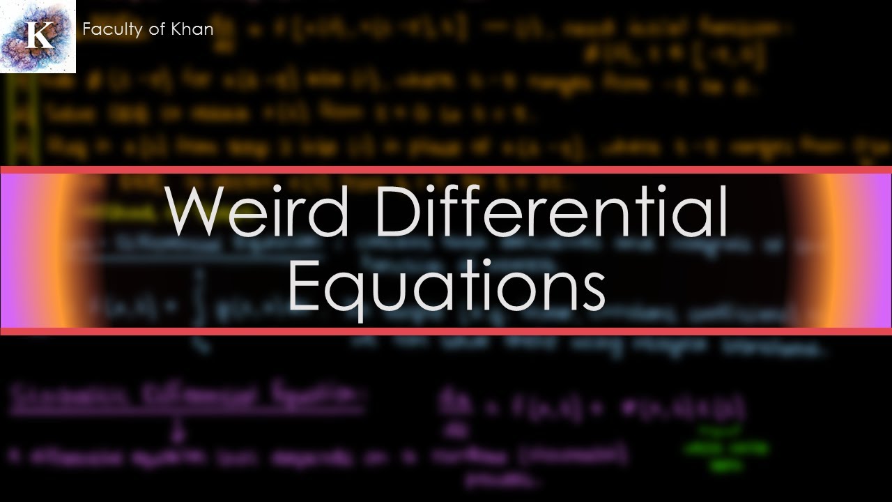
Introducing Weird Differential Equations: Delay, Fractional, Integro, Stochastic!
Overview of Differential Equations
Separation of Variables // Differential Equations
The Key Definitions of Differential Equations: ODE, order, solution, initial condition, IVP
Differential equations, a tourist's guide | DE1
Recurrence Relation | Solution of Recurrence Relation | Discrete Mathematics by Gp sir
5.0 / 5 (0 votes)