Regression and R-Squared (2.2)

Summary

This video script delves into the concept of regression and the R-squared value, explaining how they are used to measure the linear relationship between two variables. It introduces the regression line, which predicts changes in one variable based on the other, using a formula involving the slope and y-intercept. The script also covers the practical application of these concepts, including calculating the regression line for predicting a student's GPA based on study time. It concludes with an explanation of R-squared, which measures how well the regression line fits the data, indicating the percentage of variation in the dependent variable explained by the independent variable.

Takeaways

• 📈 Regression analysis involves creating a line, known as the regression line, to represent the pattern of data and predict the change in y when x increases by one unit.
• 📚 The regression line formula is y hat = b naught + (b1 * x), where y hat is the predicted value of y, b naught is the y-intercept, b1 is the slope, and x is the value of the independent variable.
• 🔍 A positive relationship between variables, such as study time and GPA, results in an upward-sloping regression line, while a negative relationship, like time spent on Facebook and GPA, results in a downward-sloping line.
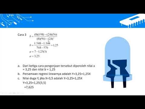
• 🧩 The values of b naught and b1 can be calculated using the formulas b naught = y-bar - (b1 * x-bar) and b1 = r * (sy / sx), where r is the correlation coefficient, and sy and sx are the standard deviations of y and x, respectively.
• 📊 To apply regression in practice, one must gather data, create a scatter plot with the dependent variable on the y-axis and the independent variable on the x-axis, and calculate the mean and standard deviations for each variable.
• ✅ The correlation coefficient (r) is essential for calculating the slope of the regression line and ranges from -1 (perfect negative correlation) to 1 (perfect positive correlation).
• 🔢 R-squared (r²) measures the proportion of the variance in the dependent variable that is predictable from the independent variable(s) and ranges from 0 (no predictability) to 1 (perfect predictability).
• 📝 R-squared can be calculated as the square of the correlation coefficient, r, and it tells us the percentage of variation in y that is accounted for by its regression on x.
• 🔑 The regression line of least squares is the line that minimizes the sum of the squares of the vertical distances of the points from the line.
• 📜 Using the regression equation, one can predict the value of y for any given value of x, as demonstrated by predicting a student's GPA based on their study time.
• 📉 A high r-squared value indicates that the regression line fits the data well, with predicted values close to actual values, while a low r-squared value suggests a poor fit and larger discrepancies between predicted and actual values.

Q & A

What is the purpose of a regression line in statistical analysis?

A regression line, also known as the line of best fit, is used to represent the pattern of data in a graph. It predicts the change in the dependent variable (y) when the independent variable (x) increases by one unit.

How is the relationship between study time and GPA typically represented in a regression analysis?

In regression analysis, the relationship between study time and GPA is typically represented as a positive relationship, meaning that as study time increases, GPA is expected to increase as well.

What is the formula for calculating the regression line?

The regression line can be described using the formula: \( \hat{y} = b_0 + b_1x \), where \( \hat{y} \) is the predicted value of y, \( b_0 \) is the y-intercept, \( b_1 \) is the slope, and x is any value of the independent variable.

What does the slope of the regression line indicate?

The slope of the regression line (\( b_1 \)) indicates the rate of change of the dependent variable (y) for each one-unit increase in the independent variable (x).

How is the y-intercept (\( b_0 \)) of the regression line calculated?

The y-intercept (\( b_0 \)) is calculated as \( \overline{y} - b_1 \times \overline{x} \), where \( \overline{y} \) is the mean of the dependent variable and \( \overline{x} \) is the mean of the independent variable.

What is the formula for calculating the slope (\( b_1 \)) of the regression line?

The slope (\( b_1 \)) is calculated as \( r \times \frac{s_y}{s_x} \), where r is the correlation coefficient, \( s_y \) is the standard deviation of y, and \( s_x \) is the standard deviation of x.

What is the significance of the correlation coefficient (r) in the context of regression?

The correlation coefficient (r) measures the strength and direction of the linear relationship between two quantitative variables. It is used in the calculation of the slope (\( b_1 \)) in the regression line formula.

How can the regression line be used to predict the value of y for a given value of x?

To predict the value of y for a given value of x, you substitute the value of x into the regression line equation and solve for \( \hat{y} \), the predicted value of y.

What is the meaning of R-squared (\( R^2 \)) in regression analysis?

R-squared (\( R^2 \)) is a measure of how well the regression line fits the data. It represents the proportion of the variance in the dependent variable that is predictable from the independent variable.

How does R-squared (\( R^2 \)) relate to the correlation coefficient (r)?

R-squared (\( R^2 \)) is the square of the correlation coefficient (r). It ranges from 0 to 1, with values closer to 1 indicating a better fit of the regression line to the data.

What does an R-squared value of exactly 1 imply about the regression line?

An R-squared value of exactly 1 implies that the regression line perfectly fits the data, meaning that it can predict the value of y for any given value of x without any error.

Outlines

00:00

📈 Understanding Regression and the Regression Line

This paragraph introduces the concept of regression, which involves creating a regression line on a graph to represent the pattern of data between two quantitative variables. The regression line predicts the change in the dependent variable (y) when the independent variable (x) increases by one unit. It explains the positive and negative relationships between variables, using study time and GPA, and time spent on Facebook as examples. The formula for the regression line is given, with y-hat as the predicted value of y, b0 as the y-intercept, b1 as the slope, and x as the value of the independent variable. The paragraph also discusses how to calculate the slope and y-intercept using the correlation coefficient (r), standard deviations of x and y, and the means of the variables. An example of predicting a student's GPA based on study time is provided, illustrating the calculation of the regression line equation and its application to make predictions.

05:01

📊 The Significance of R-Squared in Regression Analysis

The second paragraph delves into the importance of R-squared in regression analysis. R-squared measures the proportion of the variance in the dependent variable that is predictable from the independent variable(s). It is a measure of how well the regression line fits the data, indicating how close the data points are to the line. An R-squared value close to 1 suggests a strong correlation between the predicted and actual values, while a lower value indicates a weaker fit. The paragraph explains that R-squared also represents the percentage of variation in y that is accounted for by the regression on x. Using an example where r is 0.94, the R-squared value is calculated as 0.88, meaning that 88% of the variation in GPA can be explained by the study time. This metric is crucial for assessing the effectiveness of the regression model in predicting outcomes.

Keywords

💡Regression

Regression in the context of the video refers to the statistical process of fitting a line to a set of data points. This line, known as the regression line, predicts the change in the dependent variable (y) when the independent variable (x) increases by one unit. It is central to the video's theme as it illustrates the relationship between two quantitative variables, such as study time and GPA.

💡R-squared

R-squared is a statistical measure that represents the proportion of the variance for a dependent variable that's explained by an independent variable in a regression model. It is mentioned in the video to explain how well the regression line fits the data, with a value close to 1 indicating a strong fit and a value close to 0 indicating a poor fit.

💡Correlation

Correlation is a statistical term used to describe the extent to which two variables are linearly related. In the video, it is discussed to measure the direction and strength of the relationship between two variables, setting the stage for understanding the concept of regression.

💡Regression Line

The regression line is the line that best fits the data points on a scatter plot, representing the average relationship between the independent and dependent variables. The video uses the regression line to predict outcomes, such as a student's GPA based on study time.

💡Y-intercept (b naught)

The y-intercept, denoted as 'b naught' in the video, is the point where the regression line crosses the y-axis. It represents the predicted value of y when x is zero. The video explains its calculation as part of the regression equation.

💡Slope (b1)

The slope, represented as 'b1' in the script, is the rate of change of the dependent variable with respect to the independent variable. A positive slope indicates a direct relationship, while a negative slope indicates an inverse relationship, as exemplified by the video with study time and GPA versus time spent on Facebook.

💡Predicted Value (y hat)

The predicted value, symbolized as 'y hat' in the video, is the value of y estimated by the regression equation for a given value of x. It is used to forecast outcomes, such as predicting a student's GPA based on the hours studied.

💡Scatter Plot

A scatter plot is a type of plot used to visualize the relationship between two variables. In the video, a scatter plot is used to represent the data points of study time and GPA, which helps in identifying the pattern and creating the regression line.

💡Mean and Standard Deviations

The mean and standard deviations are statistical measures used to describe the central tendency and dispersion of a dataset, respectively. The video mentions these as necessary calculations for determining the regression line's equation.

💡Line of Least Squares Regression

The line of least squares regression is the line that minimizes the sum of the squares of the vertical distances of the points from the line. The video describes this as the method used to calculate the regression line, emphasizing its importance in statistical analysis.

💡Percentage of Variation

The percentage of variation accounted for by the regression on x is explained in the video through r-squared. It indicates what proportion of the variation in the dependent variable can be explained by the independent variable, highlighting the predictive power of the regression model.

Highlights

Regression is used to create a line on a graph that represents the pattern of data, known as the regression line.

The regression line predicts the change in 'y' when 'x' increases by one unit, indicating either an increase or decrease.

A positive relationship is expected between study time and GPA, as more study time generally leads to a better GPA.

A negative relationship is expected between time spent on Facebook and GPA, suggesting less study time and potentially lower GPA.

The regression line formula includes 'y-hat' for the predicted value of 'y', 'b0' for the y-intercept, 'b1' for the slope, and 'x' for any value on the x-axis.

The slope of the regression line indicates the direction of the relationship between variables.

The formula for the y-intercept 'b0' is y-bar minus (b1 times x-bar), and for the slope 'b1' it is r times the standard deviation of y divided by the standard deviation of x.

Researchers can use regression to predict a student's GPA based on the amount of weekly study time.

Creating a scatter plot is the first step in visualizing the relationship between study time and GPA for regression analysis.

Mean and standard deviations for each variable, as well as the correlation, are necessary for applying the regression formula.

The regression line equation is derived from the calculated values of 'b0' and 'b1', predicting 'y' based on any given 'x'.

The line of least squares regression is used to minimize the sum of the squares of the vertical distances of the points from the line.

The slope of the regression line in the study time and GPA example is 0.311, indicating a predicted increase in GPA for each additional hour of study.

Using the regression equation, one can predict the GPA for a student studying a specific number of hours per week.

R-squared (r²) measures how well the regression line fits the data, with values ranging from 0 to 1.

R-squared close to 1 indicates that the predicted values are close to the actual values, while a low r-squared suggests a poor fit.

An r-squared value of 1 implies perfect prediction of 'y' for any given 'x'.

R-squared also represents the percentage of variation in 'y' that is accounted for by regression on 'x'.

In the study example, an r-squared of 0.88 indicates that 88% of the GPA variation is explained by study time.

Transcripts

in this video we will be looking at

regression

and r squared when we talked about

correlation

we talked about how we can use it to

measure the direction and strength of a

linear relationship shared between two

quantitator variables

but when we talk about regression we

talk about making an actual line on the

graph

this is a line that represents the

pattern of data and this line is known

as the regression line

a regression line predicts the change in

y when x increases by 1 unit

the change in y describes either an

increase or a decrease

so for example if we have study time on

the x-axis

and gpa on the y-axis we could expect a

positive relationship between these two

variables

because generally speaking the more you

study the better your gpa will be

now if i replace study time with time

spent on facebook we could expect a

negative relationship

the regression line can be described

using this formula where y hat is the

predicted value of y

b naught is the y-intercept b1 is the

slope

and x would be any value of x if we go

back to the first example

y hat would be gpa because gpa is listed

on the y-axis

and since study time is listed on the

x-axis x is equal to any value of study

time

b naught is always equal to the y

intercept

and b 1 is always equal to the slope

notice how the slope is pointing upwards

because of this we have a plus sign

written on the formula

in contrast in this example notice how x

is now equal to the time on facebook

and like before b naught is always equal

to the y-intercept

and b-1 is always equal to the slope of

the line

this time the slope is pointing

downwards which is why we have a minus

sign written on the formula

when we mathematically examine this

formula we see that b

naught is equal to y-bar minus b-1 times

x-bar

and b-1 is equal to r times the standard

deviation of y

divided by the standard deviation of x

so let's see how we can use these

formulas in practice

suppose a researcher wants to predict a

student's gpa from the amount of time

they study each week

first the researcher needs to gather

some data

we can then begin by making a graph

since the researcher is trying to

predict a student's gpa

we will have gpa on the y-axis so by

default

gpa will correspond to the y values and

study time will correspond to the x

values

then we could choose to make a scatter

plot with this data

recall that when we are dealing with

regression we don't really care about

each individual point

we are only interested in the line that

represents the pattern of data

in order for us to use the regression

formula we need to calculate the mean

and standard deviations for each

variable

which you should already know how to do

we also need to calculate the

correlation

which you should also know how to do we

needed to calculate for these values

because b naught is equal to y bar minus

b1

times x bar and b1 is equal to r

times sy divided by sx when we solve for

the value of b1

we get 0.311 and when we solve for the

value of b naught we get a value of 1.45

therefore the equation for the

regression line will be y

hat equals 1.45 plus 0.311

times x this means that the value of the

y-intercept

corresponds to 1.45 and the value of the

slope

corresponds to 0.311

when you calculate a line using this

formula it can also be called the line

of least squares regression

the slope of a regression line predicts

the change in y

when x increases by one unit so in our

example the slope is equal to 0.311

therefore we see that as study time

increases by 1 hour

we predict a student's gpa to increase

by 0.311

we can actually use this equation to

predict the value of y

using any value of x for example

based on this data if we have a student

who studies for 6.5 hours a week

we can predict this student's gpa all we

do is plug the value 6.5 into the

formula

and we get a y-hat of 3.47

this means that for someone who studies

for 6.5 hours a week

we predict their gpa to be equal to 3.47

the last thing i want to talk about is r

squared r squared is literally equal to

r squared

or r times r do not get confused between

r and r squared r has values between

negative 1

and positive 1 whereas r squared only

has values between 0

and 1. correlation measures the linear

relationship between two quantitative

variables with respect to direction

and strength on the other hand r squared

is a measure of how close each data

point fits to the regression line

so in fact r squared tells us how well

the regression line predicts

actual values let me show you what i

mean by this

consider this scatter plot each blue dot

represents an

actual value and from this data we can

make a regression line

now any point that falls on the

regression line corresponds to a

predicted value

so in general an r squared that is close

to 1

tells us that the predicted values and

the actual values

are close together in contrast a low

value of r squared

tells us that the regression line

doesn't fit the data that well

and we can clearly see a large amount of

distance between the actual values and

the predicted values

and if r squared is exactly equal to 1

this

means that we can predict the value of y

for any given value of x

note that r squared also tells us the

percentage of variation in y

that is accounted for by its regression

on x

so in our previous example we had

calculated r to be 0.94

the r squared value would be equal to r

times r

or 0.88 so this tells us

that 88 of the variation in gpa

is accounted for by its regression on

study time