AWS DevDays 2020 - Deep Dive on Amazon SageMaker Debugger & Amazon SageMaker Model Monitor

Summary

This session delves into Amazon SageMaker's advanced capabilities, focusing on SageMaker Debugger for monitoring model training and Model Monitor for detecting data and prediction quality issues post-deployment. The speaker demonstrates using these tools with a classification model, highlighting features like data capture, real-time analytics, and automated rule-based checks to ensure model reliability and efficiency. Additionally, cost optimization strategies for SageMaker are discussed, including spot instance training and model tuning for efficient resource utilization.

Takeaways

• 📘 The session focuses on Amazon SageMaker's capabilities, specifically the Debugger and Model Monitor features, which assist in inspecting model training and identifying data quality issues post-deployment.
• 🛠️ Amazon SageMaker Debugger allows users to save model states, such as tensors representing the model's parameters, gradients, and weights, periodically during training to S3 for later inspection.
• 🔍 Debugger's rules can be configured to monitor for undesirable conditions during training, such as class imbalance or vanishing gradients, providing real-time feedback and potentially stopping the training job if issues arise.
• 📊 SageMaker Debugger can visualize feature importance, helping to understand which dataset features contribute most to the model's predictions, enhancing model explainability.
• 🔄 The session demonstrates using spot instances for training models on SageMaker to save costs, with significant savings shown in the example.
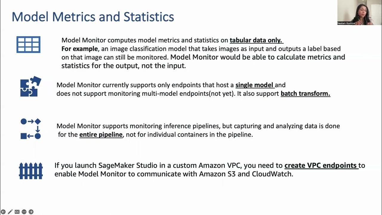
• 📈 Model Monitor captures data sent to a model in production, including requests and predictions, storing this information in S3 for analysis and monitoring data quality over time.
• 📉 Model Monitor can detect data quality issues such as missing features, mistyped features, or drifting features, which may degrade prediction quality if not addressed.
• 📝 The speaker emphasizes the importance of cost optimization in using SageMaker, covering topics like using managed services, spot training, and elastic inference to reduce expenses.
• 📚 The session mentions various resources for learning more about SageMaker, including documentation, AWS blog posts, YouTube videos, and podcasts, encouraging attendees to explore these for further insights.
• 🚀 The speaker highlights the productivity improvements offered by SageMaker Debugger and Model Monitor, suggesting they can save users significant time and frustration in model development and monitoring.
• 🗓️ The session ends with an invitation for attendees to ask questions, indicating the speaker's availability for further discussion and assistance on Twitter.

Q & A

What is the main focus of the session on Amazon SageMaker?

The session focuses on Amazon SageMaker Debugger and Model Monitor, explaining how they help in inspecting model training and finding data quality and prediction quality issues once models are deployed.

Where can the slides and recording of the session be found?

The slides can be found in the handout tab on the control panel, and the recording will be sent in a follow-up email after the event.

What is the dataset used in the notebook for training the model?

The dataset used is a direct marketing dataset, which is a supervised learning problem classifying customers into two classes based on whether they accept an offer or not.

What is the purpose of using spot instances in SageMaker?

Spot instances are used to save money on training costs. They allow users to specify a maximum training time and a total time, including waiting for spot instances, to control how long they are willing to wait for spot instances.

How does SageMaker Debugger save model information during training?

SageMaker Debugger saves tensors, which are high-dimensional arrays representing the state of the model, periodically during the training job. This model state is saved to S3.

What is the purpose of defining rules in SageMaker Debugger?

Rules in SageMaker Debugger are used to check for unwanted conditions during the training job. They can be built-in or custom Python code to inspect tensors and ensure the training job is not suffering from issues like class imbalance, vanishing gradients, or exploding tensors.

How can feature importance be visualized using SageMaker Debugger?

Feature importance can be visualized by accessing the specific tensor by name, getting all the steps, and then plotting the values for each step using a tool like matplotlib.

What is the role of Amazon SageMaker Model Monitor in the session?

Amazon SageMaker Model Monitor helps in capturing data sent to the model in production, saving incoming and outgoing data (request and response) to S3, and running analytics to detect data quality and prediction quality issues.

How can baseline statistics be generated for Model Monitor?

Baseline statistics are generated by uploading the training set to S3 and creating a baseline using SageMaker Processing. This process computes statistics on the training set, such as feature types, ranges, distributions, and constraints.

What is the significance of creating a monitoring schedule in Model Monitor?

A monitoring schedule in Model Monitor is used to periodically analyze the captured data and compare it with the baseline statistics. It helps in detecting discrepancies and alerting to problems like missing features, mistyped features, or drifting features.

What are some cost optimization strategies mentioned in the session?

Cost optimization strategies include using managed services like EMR or Glue, stopping and sizing notebook instances appropriately, using local mode, managing spot training, optimizing models with Model Tuning Autopilot, using Elastic Inference, and leveraging inference with custom chips for high-throughput prediction.

Outlines

00:00

📘 Introduction to Amazon SageMaker Debugger and Model Monitor

The speaker introduces the session on Amazon SageMaker, focusing on the Debugger and Model Monitor features. They explain that the Debugger helps to inspect model training processes by saving tensors and model states to S3, which can later be analyzed for issues or metrics plotting. Model Monitor is highlighted for its ability to detect data and prediction quality issues post-deployment. The session promises an in-depth look at these tools using a notebook available on GitHub, with a practical example of building a classification model on a direct marketing dataset. The speaker also mentions the availability of slides and a recording for future reference.

05:02

🔍 Setting Up SageMaker Debugger for Model Training

The speaker details the process of setting up SageMaker Debugger for a training job. They explain how Debugger saves model information such as tensors, parameters, gradients, and weights during training to S3. This feature allows for the inspection of the training job for any undesirable conditions or analysis of metrics. The speaker demonstrates how to configure Debugger by defining tensor collections and setting a save interval. They also discuss the use of built-in rules to monitor for specific conditions like class imbalance during training, using a real-world example of a highly imbalanced dataset.

10:04

🚀 Launching the Training Job with Debugger and Model Monitor

The speaker proceeds to launch a training job with the configured Debugger settings. They describe the process of setting hyperparameters and initiating the training job, while emphasizing the cost-saving benefits of using spot instances for training. The speaker explains how the Debugger runs in parallel with the training job, checking for predefined rules and saving model states to S3. They also mention the ability to stop the training job if a rule is triggered, to prevent wasting resources on a failing job.

15:05

📊 Analyzing Model States and Tensors with SageMaker Debugger

After the training job is completed, the speaker explains how to explore the saved tensors in S3 using the SageMaker Debugger SDK. They demonstrate how to access and plot the history of specific tensors over the training steps, using the area under the curve (AUC) as an example metric. The speaker also shows how to analyze feature importance to understand which features contribute most to the model's predictions, using a plot to visualize the importance of different features.

20:06

🌟 Advanced Use Cases of SageMaker Debugger

The speaker provides an overview of advanced use cases for SageMaker Debugger, such as model pruning, where unnecessary parts of a deep learning model are removed during training to reduce model size without significantly impacting accuracy. They highlight the extensive examples available in the SageMaker GitHub repository, which showcase how to utilize Debugger for deep insights into model behavior and performance.

25:08

🔎 Implementing Data Capture with SageMaker Model Monitor

The speaker shifts focus to SageMaker Model Monitor, starting with its data capture functionality. They explain how to enable data capture when deploying a model, which involves saving incoming and outgoing data to S3 for analysis. The speaker demonstrates capturing data by sending test samples to a real-time endpoint and shows how the captured data can be accessed and analyzed.

30:10

📈 Establishing a Baseline for Model Monitor

To utilize Model Monitor effectively, the speaker describes the process of establishing a baseline using the training dataset. They explain how to upload the training data to S3 and use SageMaker Processing to compute statistics and constraints that define what 'clean' data looks like. This baseline is crucial for later comparison with real-world data to detect discrepancies.

35:13

🚨 Detecting Data Drifts with Model Monitor

The speaker discusses how Model Monitor can detect data drifts by comparing incoming data against the established baseline. They demonstrate setting up a monitoring schedule to periodically analyze the captured data for deviations from the training set. The speaker also simulates data corruption to illustrate how Model Monitor can alert users to such issues, pointing out the importance of this feature in maintaining model accuracy over time.

40:14

🛡️ Cost Optimization Strategies in SageMaker

Towards the end of the session, the speaker touches on cost optimization strategies in SageMaker. They mention various techniques such as using managed services for data preparation, stopping and sizing notebook instances appropriately, leveraging spot training, and considering elastic inference for deployment. The speaker encourages attendees to read a detailed blog post on cost optimization for more insights and to share any additional techniques they might have.

📚 Additional Resources and Closing Remarks

In the final part of the session, the speaker provides a list of resources for further learning, including the SageMaker documentation, AWS blog posts, a Medium blog, a YouTube channel, and a podcast. They invite attendees to follow them on Twitter for more updates and assistance, emphasizing their openness to answering questions and providing guidance on SageMaker and related topics.

Keywords

💡Amazon SageMaker

Amazon SageMaker is a fully managed service that provides developers and data scientists the ability to build, train, and deploy machine learning models quickly. It is central to the video's theme, showcasing its capabilities in model training and monitoring. The script discusses using SageMaker for training models, debugging, and monitoring, highlighting its efficiency and integration with other AWS services.

💡Debugger

In the context of the video, 'Debugger' refers to SageMaker Debugger, a feature that enables developers to inspect and understand the model training process by saving model states and analyzing tensors. It is a key concept as the script delves into how Debugger can help identify issues such as class imbalance or vanishing gradients during training, using rules to monitor for undesirable conditions.

💡Model Monitoring

Model Monitoring is another core concept in the video, referring to the capabilities of SageMaker Model Monitor. It helps in detecting data quality and prediction quality issues post-deployment by capturing and analyzing data sent to the model in production. The script explains how it can be used to ensure the model's predictions remain accurate over time by monitoring for data drift or other anomalies.

💡XGBoost

XGBoost, short for eXtreme Gradient Boosting, is an optimized distributed gradient boosting library designed to be highly efficient, flexible, and portable. In the script, XGBoost is used as an example algorithm for building a classification model on the direct marketing dataset, demonstrating SageMaker's support for popular machine learning frameworks.

💡Direct Marketing Dataset

The Direct Marketing Dataset is a real-world dataset used in the script to illustrate the process of training a classification model. It classifies customers into two categories based on whether they accepted an offer or not. The dataset is used to demonstrate the practical application of SageMaker's capabilities in a supervised learning context.

💡Spot Instances

Spot Instances in the video refer to Amazon EC2's spare computing capacity offered at a discounted price. The script mentions using Spot Instances for training machine learning models in SageMaker to save on costs, highlighting the cost-effectiveness of using such instances when the model training time is flexible.

💡Feature Importance

Feature Importance is a concept discussed in the script that helps in understanding which features in the dataset contribute the most to the predicted outcome. It is illustrated through the use of SageMaker Debugger, showing how it can be used to analyze the impact of different features on the model's predictions, enhancing model explainability.

💡Data Capture

Data Capture is a functionality of SageMaker Model Monitor that is explained in the script. It involves saving the incoming and outgoing data (requests and predictions) sent to a deployed model's endpoint to S3 for later analysis. This feature is crucial for auditing, debugging, and understanding the performance of the model in production.

💡Baseline

In the context of model monitoring, a 'Baseline' is a set of statistical properties derived from the training data that serves as a reference point. The script explains how a baseline is created using SageMaker Processing and then used to compare against real-world data to detect discrepancies, which is essential for identifying data drift or other issues affecting model performance.

💡Elastic Inference

Elastic Inference is a service mentioned in the script that allows for cost-effective inference by sharing a GPU across multiple instances. It is part of the broader discussion on cost optimization in machine learning workflows. The script suggests that Elastic Inference can be a more cost-efficient option for deploying models compared to using full GPU instances.

Highlights

Introduction to Amazon SageMaker Debugger and Model Monitor for inspecting model training and deployed model performance.

Amazon SageMaker Debugger helps in saving model information and inspecting tensors during training.

Demonstration of using the XGBoost algorithm to build a classification model on a direct marketing dataset.

Explanation of basic data preprocessing and uploading datasets to Amazon S3 for training, validation, and testing.

Utilization of an estimator for model training with Amazon SageMaker, including the use of spot instances to save costs.

Configuration of SageMaker Debugger to enable model state saving and rule checking during training.

Use of built-in rules in SageMaker Debugger to monitor for issues like class imbalance during training.

How to access and plot model metrics and feature importance using the SageMaker Debugger SDK.

Example of using SageMaker Debugger for model pruning in deep learning to optimize model size and performance.

Introduction to SageMaker Model Monitor for capturing and analyzing data sent to models in production.

Setting up data capture on a SageMaker endpoint to record incoming and outgoing data for analysis.

Creating a baseline for data using training set statistics to compare against real-world data for discrepancies.

Using a monitoring schedule to periodically check for data quality issues in production model data capture.

Detecting and reporting data violations that differ from the training set baseline with Model Monitor.

Cost optimization techniques for SageMaker, including managed services, spot training, and elastic inference.

Resources for further learning on SageMaker, including documentation, blog posts, YouTube channel, and Twitter.

Transcripts

hi everyone welcome to this new session

on Amazon sage maker if you have any

questions please submit them the

questions pane on the control panel and

I will answer them at the end a copy of

the slides can be found in the handout

tab on the control panel and you will

get a copy of the recording in a

follow-up email after the event in this

session I'm going to dive even deeper on

sage maker and this is actually 0 slides

or almost and we're going to talk about

Amazon sage maker bottle debugger and

how it helps inspecting what's going on

during model training and then we'll

look at Amazon sage maker model monitor

which helps you find data quality and

prediction quality issues once your

models have been deployed okay so let's

jump straight into the notebook this

notebook is available on github and here

I'm going to use the XJ boost I'll go to

build a classification model on the

direct marketing data set so I'm not

going to dive too deep on the data set

and and the problem we're trying to

solve I'm actually going deeper into

this in the next session which is more

obsessed about performance and accuracy

here we want to inspect and and and

monitor so it's not so much about

getting great accuracy so in a nutshell

this is a direct marketing dataset it's

a supervised learning problem

classifying customers into two classes

customers who accept an offer customers

who don't okay so kind of a yes or no

problem so the first step is to download

the data set extract it and we can take

a look with pandas right so it's a CSV

file a bunch of features and a why

column saying yes or no

did the customer accept the offer okay

then I'm doing some some basic

pre-processing but again I'm not going

to to look at this now because I'm not

concerned with this at the moment so

basic processing then complete the data

set and and upload everything to s3

okay so I have a training set I have a

validation set and I have a test set

okay and I have the three locations for

those three data sets okay so now we

want to train a model okay so if you

work with sage maker before you know

this means using an estimator okay

I'm using a built in I'll go here so I'm

using this estimator object which is the

the generic I'll go for for built in

sorry the generic so I'm using the

estimator object which is the generic

object for built-in algos first

I grab the name of the container image

for XJ boost in the region I'm running

in and I am configuring the estimator

and yes it is quite a mouthful because I

try to fit as much as I could in there

so we're going to take it step by step

let's look at the bits that we probably

already know okay so the bits we all

probably already know are these right we

need to pass the name of the container

so basically selecting the algo we want

to we want to use we pass an IM role to

give stage maker permissions to access

s3 pool docker containers etc etc the

session which is a technical object then

we use file mode to say want to copy the

data set to the instance before training

we define the location the output

location for the model and we define how

much infrastructure we want okay so here

we're training on one ml and for 2xl

instance okay

so if you work with say drinker before

and even if you haven't I guess you know

these are very simple very reasonable

okay

the next bit is about using spot

instances

okay so spot instances are a great way

to save money they've been available on

ec2 for a long time they are now

available on Sage maker so just say hey

I want to use spot instances for

training my max training time is this

and my total time so training time plus

waiting for spot is this okay

so that's how you control how much time

you're ready to wait for spot instances

if they're in really high demand okay

fine so let's look at the next bits okay

so the next bits are actually new stuff

let's look at this one first okay so

this is the debugger configuration okay

and as you can imagine this is an object

coming from the sage maker debugger is

DK okay and this is how we're going to

enable sage maker debugger for this

training job okay so let me explain what

sage maker debugger does so what it does

is as your job is running it's going to

save model information so tensors okay

tensors are high dimensional arrays that

represent the state of the model

parameters gradients weights if you use

deep learning etc and that model state

is going to be saved

periodically during the training job and

of course it's going to be saved to s3

as you can see here okay so the high

level idea is we save that stuff

periodically to s3 okay and later on

we're going to be able to look at it

okay and understand what happened in

that training job

potentially looking for bizarre

conditions or just you know plotting

metrics and whatnot okay so that's a

super easy way to save model state

periodically okay and that's what we see

here so we define collections for the

different tensors so we have metrics and

of course these are predefined A's

we have feature importance that's a

really nice one as we'll see telling us

which features in the dataset

contribute the most to the predicted

outcome by XJ boost and then we pass the

save interval okay so do we want to save

at every step or every five steps or ten

steps so here I'm saving all steps

literally saving everything okay so

that's what we're doing here

and we'll see how this actually happens

but this is how you configure it this is

how you configure the saving part of the

program okay but it's not just about

saving okay it would be nice already

free if we were able to to look at that

model state after training is complete

but we can actually define rules okay so

we can actually ask sage maker debugger

to check for unwanted conditions during

the training job so we have a list of

built-in rules that you'll find in

documentation and you can add your own

okay so you could write your own Python

code to inspect your tensors and check

for you know weird stuff happening there

so here I'm using a rule a built in

recalled class imbalance because as it

turns out this is a very imbalanced data

set about eight to one and well building

classifiers for imbalance states that is

more difficult okay so I want to make

sure that these training jobs not

suffering from that imbalance rule

and I could further configure this but

you'll find this information in the in

the doc okay so here I'm just saying hey

keep your keep an eye out for class

imbalance weirdness

during the training job and and use that

stuff to look at metrics basically okay

so that's what sage maker debugger does

okay one it will save define tensor

collections to s3 so that you can

inspect them okay to it configures rules

that are checked during training okay to

make sure your training jobs not

suffering for from something undesirable

and and just weird

okay so just on the top of my mind you

can check for you know lost not

decreasing and vanishing gradients and

exploding tensors and a whole bunch of

things yes they all have very funny

names okay so please take a look at the

doc for more alright so this is my

estimator okay

the usual part and more stuff for

debugger okay next I'm just setting some

hyper parameters okay and as you can see

I'm actually very reasonable here for

once I am NOT setting any crazy ones

because once again I am not really

trying to get to a high performance

model here I'm just trying to show those

those new capabilities if you're curious

about optimizing hyper parameters etc

that's the next session okay so don't

miss it okay and then I co fit and my

training job starts okay let's take a

look at the log so we see the usual

stuff start the training job launching

instances etc and we see new stuff as

well okay we see debugger rule status

class in

in progress so and then we see pretty

much though the training job as usual so

what's this bit so what this means is

based on the configuration above okay

here we can figure one rule well we see

sage record firing up in parallel of the

training job another job for that

debugging rule okay and we we have one

job Peru so if we'd configured let's say

five debugging rules then we would see

five debugging jobs okay and as you can

imagine what these jobs do is they look

in real-time as they become available

they look at the tensors that are saved

in s3 and they check for whatever

condition they've been set up for okay

so there's code looking at tensors and

applying that logic trying to figure out

yes or no is class imbalance a problem

or it's lost not decreasing etcetera

etcetera okay so that's a separate job

running in parallel okay alright so we

see our job we see very nice savings

from spot okay so 66.7% that's very nice

we saved two thirds of the on the

training cost so make sure you know how

to use spot instances and decrease your

say check your bill okay we'll talk

about cost optimization some more at the

end as promised in the session

description but as you can see spot is

already a very nice way to save money

okay I can check the condition of that

debugging job

as the training job is going okay so

here when I check was in progress now

for sure it's done and if something

happens which I don't think happen here

if the rule is actually triggered then

the debugging job stops and your

training job stops as well be

there's really no point in continuing

training if something is not going well

it's just a waste of time and money so

if a rule is triggered then the

debugging job will let you know

something went wrong and and the

training job the corresponding training

job will be stopped

okay so no need to if you have vanishing

gradients for deep learning job that

train for seven days well you know you

might as well save that time and money

okay so once the job is over so whether

it successfully completed or not you can

go and explore those stances in s3 okay

and you need to do that using that SDK

for SM stage maker debuggers debugger

basically find the path for the artifact

so basically where did we save the

tensors and then create a trial from

from that okay and once you have that

then you can start exploring your data

okay so there's not enough time to cover

the the full api of the the trials SDK

but again all the documentation is

online but basically you can see you can

access a specific tensor by a name and

you can get all the steps okay remember

we save data periodically okay so you

can get the tensor values for every step

and and then you get here we're building

as you can see we're building a Python

list and returning a list of steps and a

list of values okay so we we have

basically only history for that tensor

over time okay and we can plot it using

matplotlib so here's an example okay

where we plot for that trial we plot our

metrics so we can see in that metrics

collection we actually had two

individual values we had the area under

curve which was the

the metric configured for that training

job and we have that for the training

set and we have that for the validation

set okay so we can see all the values

over time and and that's already very

useful right pretty easy to do that okay

and I guess we could have continued

training for a bit more or not but

doesn't matter at this point okay so you

can easily access just like that okay

basically those those two three lines

okay access tensors by name and get all

their steps and get all the values for

the steps okay again full history over

those model model values and model

states okay so that's pretty cool you

don't need to write any bespoke code to

do that

remember we saved another collection we

saved feature importance okay so feature

importance once again will tell us which

feature contributes most to the

prediction okay and our our data set

here as sixty plus features because we

use a one heart and coding on

categorical variables etc so it's

actually much more than the 20 columns

we have originally and and we can see

that okay so if we plot that then we see

that feature okay the orange one I

believe is this one f1 ok and this one

is f5 okay so we see that feature 1 and

peach 5 are the important ones okay

which is good because that's exactly

what the comment says here and so future

one is actually the job it's the number

of the column right in the in the CSV

file so there's no well there's no magic

on those numbers so does that person

have a job and

how is it housed is it you know is it

renting or is that person renting or is

that person owning and these are I guess

important factors in you know how much

money you can generally spend so so not

surprising to see them as highly

contributing to whether you would accept

a marketing offer or not okay so this is

really really cool because you certainly

heard about model explain ability well

this is it right so if you train the

classification model and you see that

okay job and housing are important

factors then you can compare that to the

to the legacy solution that you have

maybe it's an IT application or maybe

it's just humans looking at forms and

deciding yes or no should they get you

know should they get that offer and you

know it helps you understand what's

going on inside the model okay and this

is super easy just save the chancers and

and just plot that stuff okay again

there are some additional details here

on future importance and it's all in the

doc but you can see just copy paste that

code it will work out of the box with

with your own model okay so there you

there you are that's a first example of

sage maker debugger okay so you can do

much more I'm just gonna give you a

taste of what's possible here and I'm

gonna jump to the Amazon sage maker

examples repository on github which is

amazing and it has hundreds and hundreds

of notebooks showing you how to use sage

maker in all kinds of ways and there's a

specific directory here for sage maker

debugger and well I have to say these

are even more amazing honestly I'm still

going through some of those but here you

see you know how deep

down you can go and literally rip the

guts of your model and and there are

some really amazing examples on deep

learning right so if you want to look at

one of them I guess we can maybe take a

look at this one really quickly so this

one shows you how to do model pruning so

model pruning is an advanced technique

where during training you look at deep

learning connections right so neuron

connections and you figure out how much

they contribute to the output so it's

kind of similar to that feature

importance example that we saw except

here we go one step further and we say

hey if a certain filter if a certain a

convolution operation does not

contribute to to the outcome then we

remove it okay so this is an amazing

notebook and I'll just go all the way to

the end okay and this this animation

here shows you over time over ten

iterations that you know we keep

removing parameters in that deep

learning model okay it's a PI torch

model and of course we shrink the model

accordingly right we go from 200 plus

Meg's to you about 70 Meg's and we

hardly lose any accuracy so we shrink

the model by a factor of three and we

hardly lose any accuracy because we just

drop parts of the of the model that just

do nothing for us okay so this is a very

very advanced example and if you're into

deep learning and computer vision I mean

yeah you're gonna love this one but not

all of them are as hardcore at ease we

have some extra boost examples as well

we have some you know slightly slightly

easier ones but again if you want to

really really dive deep on on sage maker

debugger just go check those notebooks

spend time to read the code and run them

and and again you'll be able to tear

your model apart sand and understand

exactly what's going on okay so really

really cool stuff here okay

so that's that's it for stage maker

debugger we could spend you know hours

on this but hey I'm I'm limited for time

ask me your questions happy to answer

questions after after the session okay

so we saw how to save model state

inspect expected etc now let's talk

about another capability which is sage

American model monitor okay so sage make

your model monitor will help us do two

things first it's gonna help us save

data that is sent to our model in

production okay so let's say we deploy

the model on a real-time endpoint and

we're able to capture data sent to that

endpoint and we're able to capture

predictions okay so incoming and

outgoing data request response if you

will save everything to is three and

look at it run analytics etc and we're

gonna be able to do much more but I'm

gonna keep some some tension here let's

just look at capturing data first so

going back to the model that I trained

I'm going to call deploy on that

estimator as usual okay

give an endpoint name give some

infrastructure requirements and AHA

there's new stuff again we pass the data

capture config coming from here okay

from the model monitor SDK and what do

we say here we say hey please capture

okay

yes that kind of makes sense please

capture everything okay 100 percent of

data right you could sample down if you

want it

by default we are going to capture

incoming and outgoing data so there are

samples and predictions and we're going

to put all that stuff in s3 here okay

very simple object okay so as you can

see here we are enable data capture at

deployment time but if you have an

existing endpoint you can do the same

okay all you have to do is you create a

new endpoint configuration with a data

capture config object and you update the

endpoint configuration with that new

with that you endpoint okay so that's so

that's all it takes right all right

after a few minutes this is live and

it's an endpoint so we can send it some

data right so just loading some test

samples using the invoke endpoint API

from boto 3 sending data getting

predictions back okay now this is just

an excuse to to log some stuff of course

ok and if I look in my capture path I

can see files right so I can see our

file here ok

adjacent lines file containing incoming

and outgoing data and I can copy it to

my local notebook instance and I can

take a look at it ok and well what do we

see exactly what we thought we'd see I

suppose we see input data which is CSV

data right and then I see my my data

point here all the way through here ok

my features and then I see the output ok

and the output is basically the 0 to 1

probability for that sample ok remember

it's a binary classification model so we

get a probability between 0 and 1 ok and

we see how a whole bunch of that ok

so again this is already very useful

because you know if you want to to

monitor our data if you want to capture

data and replay it right if you want to

do back testing you could say well okay

let's capture real real life data and we

can replay that stuff in a damn or test

environment you know no code to write

the only thing that we've done was that

data capture config object on on the

endpoint right so this is already pretty

nice okay and then we do bat prediction

because why not okay and that's it okay

so this is the capture part right but

model monitor actually goes a little

further than this okay and once again

let me show you more examples so in that

same repo okay say to make sure examples

you have a directory for model monitor

and you have some examples here and I'm

gonna show you a little bit more because

I have a little bit more time okay so in

this notebook we're actually using a

different data set but again it doesn't

really matter we can just focus on on

the model monitor part so what we do

here is actually we take an existing

model okay this is a turn partition

model so probably again a binary

classifier a model that has already been

trained okay and we import it we deploy

it on sage maker we set up data capture

exactly the same way capture everything

we deploy it right and this is a good

example of the modularity of sage maker

see we're just taking a model that you

could have trained on on another machine

on your laptop baby and you can very

easily deploy it on sage maker okay then

we send it some data okay just like

we've done in the previous example we

see capture file

we can see what's inside those files

okay so Jason lines format

exactly the same all right so this is

really what I've done in my previous

example but again we can go further we

could say okay so we have data capture

we have that stuff ready to ready to run

and actually already running so now we

can say well it'd be nice if we could

compare incoming data

okay real life data sent to my endpoint

to the data that I use to train the

model okay and well you can absolutely

do that so the first step is to generate

a baseline okay so generating a baseline

means you're going to compute some

statistics using the training set okay

so here we upload the training set to s3

and we create a baseline okay so we

launched a specific job that will load

the training set as you can see here and

it's going to compute all kind of

statistics on it it's going to figure

out feature types feature ranges feature

distributions etc etc okay if you're a

data scientist you certainly do that

manually already okay but here you can

automate that okay so we can see that

job running here and by the way this is

based on another sage make your

capability go sage maker processing that

makes it easy to run scikit-learn or

SPARC processing jobs on data and you

can use it in many different ways

pre-processing data or computing stats

or you know running batches of a batch

processing on your data pretty much okay

that's a service in itself but hey it's

integrated here okay so just compute

that baseline and it runs for a bit okay

let's not look at that okay and once the

job is over we can see some results so

we can see statistics on the data and

constraints okay and basically what that

means if we look at that data here we

can see for each feature what type it is

okay

is it an inner girl is it is it a float

or is it something else

we can see if we have missing values for

that feature okay so apparently not okay

we have all features are present in our

examples we can see stats okay so we see

distributions using kll if you do that

stuff for a living you know what I'm

talking about if not I don't worry about

it it's just a very fast way to compute

distributions and there's a whole lot of

stuff here

right so if you're into statute of love

this a mean standard deviation etc etc

okay all that stuff is just automated

away okay

and now that we know what clean data

looks like okay hopefully the data set

is a clean one of course we can compare

incoming data to that okay and the way

we're gonna do this is we're going to

create a monitoring schedule which is

going to look at captured data remember

okay we're capturing incoming data and

it's going to look periodically at that

data and it's going to run those same

statistics okay and constraints on that

incoming data and it's going to look for

our discrepancies okay it's going to

look for differences so if everything is

fine then okay

things are not fine that's gonna tell us

and so this is going to alert us to

problems like missing features mistyped

features are drifting features which are

even worse where the distribution of a

feature is now different because

whatever you know because the real world

is ever changing and I think we have

good proof at the moment so maybe the

hypothesis that were true on your data

set a month ago are not true anymore

and of course this would mess with your

predictions very badly because all those

machine learning algorithms use

statistics and distributions so if those

hypotheses are you know shifting then

predictions will shift and and the

quality of your predictions are going to

degrade over time okay and this is a

very nasty problem and it's very

difficult to track yes maybe you see

your business KPI going down because

your predictions are not so relevant but

why you know why is that KPI going down

well okay this could be one of the

reasons okay and of course you could

just be bugs right maybe something in

your ETL workflow is broken and and all

of the sudden you know data is not it's

not what it should be or maybe a web app

upstream is just you know it's just

buggy and and dropping features or

adding extra crappy features whatever

you know it's software anything can

happen and and all of it would impact

your models so that's that's not very

good okay so that monitoring schedule is

what is going to fix that for you okay

all right so next we're going to start

generating traffic and and of course we

break it on purpose okay and we break it

on purpose

because we're applying buggy

pre-processing to to that day

okay so so this is buggy code that

arbitrarily and randomly breaks incoming

data okay so take a look at that and so

that traffic is gonna be it's gonna be

bad that traffic right it's gonna be

garbage and so after a while you know

once or monitoring schedule kicks off

okay and of course here I think we have

a already schedule but you can you can

configure that so after an hour it's

gonna it's gonna fire up and and of

course it's going to crunch the data

that we captured and again remember this

is bad data because we literally broke

it for testing purposes and we then see

that oh that Marlin monitoring schedule

did run but and it completed but it

detected violations so violations are

basically data that doesn't look like

the training set okay which is what we

want here we broke it okay so we can go

and grab the reports for those

monitoring schedules and there is a

violation report which we can visualize

and here well what did we do well I

guess we broke yeah so we expected

integers and maybe we did pass strings

or something so I think we you know we

messed up we messed up a number of

features yeah in the processing script

and these are picked up okay

so again this is just one of the

violation here we just messed with the

datatype but if you had different

statistical properties those would be

highlighted as well okay so this is a

really really cool capability if you ask

me because it it just runs in the

background you know and it will catch it

will catch that stuff and and then you

can go and look at those and try to

understand okay

is that my ETL chain you know messing

with my data or did a feature disappear

from my data set because maybe you know

maybe my web app is not logging it any

longer you know it basically points you

at the the problem and then you can go

and investigate more but at least you

know what to look for you know what was

wrong in that sample that you received

okay and then you can you know you can

start and start your schedules and you

can delete them if you want just so you

know you can't delete an endpoint you

feel as an active monitoring schedule so

you need to make sure if you get that

error you need to delete the monitoring

schedule first and then you'll be able

to delete the endpoint okay all right

well I think that's it for for model

monitor and again we have more more

notebooks here and including

visualization etc etc so both these

debugger and model monitor our notebooks

are really really awesome so spend some

time you know read documentation first

go through the basic examples and then

you can dive deep into that and and set

this up and both capabilities really

will save you so many hours of

frustration trying to understand why

it's your training job not going right

and why is my model not predicting right

and these are great great productivity

improvements and and we get a really

good feedback from customers so well

please try them out and let us know okay

just just a few more things I promised I

would talk about cost optimization for a

second so the reason why I'm including

this in these sections because usually I

see a lot of customers who you know

first they try to get a hang of sage

maker and then they get protective and

they deploy and they really love the

fact that they can launch all that

infrastructure and amount etc etc and

and then you know it scales very nicely

but if you don't pay attention then you

could end up spending a little more

money than you expect it okay so you

have to be careful there and and I wrote

a blog posts over a year ago already but

it's been a dated post reinvents with

all the new launches and and this is on

my medium blog and i pretty much walk

through all the steps so data

preparation using manage services like

my EMR instead or glue which is a really

cool tool for machine learning as well

instead of trying to write your bespoke

code on ec2 ground truth for labeling

which will save you lots of time and

money and then you know and working with

notebook instances right stopping them

when you don't need them right sizing

them using the local mode I mean if

you've never heard of all those things

if local mode means nothing to you then

you're probably spending too much money

okay so go through that blog post check

all the boxes and and send me a tweet

telling me how much money you saved okay

managed spot training we saw is a

fantastic way to save you know easily 60

70 percent on training jobs again

right-sizing working with your data set

in the right format streaming with pipe

mode again if you have large data set

and you've never heard of pipe mode

please take a look I have a really

fantastic guest post from hime-chan's

an engineer with mobile I working at

very large scale tensorflow and they

this is really you know all the

knowledge you need on pipe mode then

optimizing models model tuning autopilot

optimizing prediction etc etc so as you

can see there are so many things you can

do

optimization elastic inference okay if

you deploy on GPU instances and you

never looked at elastic inference I can

pretty much guarantee that you're you

know probably wasting quite a bit of

money so take a look here inferential is

a great it's a great new capability as

well with a custom chip for a super high

throughput prediction you know much more

efficient than GPUs etc etc right the

list goes on and I keep updating this

post every time so long story short if

you've never worried about cost

optimization and you know even if you're

working at small scale and if you're

working with GPU and Stasi etc please

take a look at this blog post I got a

lot of good feedback on it and you know

I want you to spend exactly what you

need to spend and not a penny more so so

please read this if you have other

techniques to share happy to add them to

the post again lots of money to save if

you do things right here okay all right

I think we're almost done so if if you

want more content well of course you can

go and read the sage maker documentation

but I guess you figure that out I have

plenty of machine learning blog post on

the AWS blog and that's a good way to

keep an eye out for new stuff because

there will be new stuff all the time my

medium blog which I just showed you my

youtube channel where there's a quite a

bit of sage maker videos and the video

version of my podcast as well the audio

podcast is on Buzz proud and I'm always

happy to to chat and answer questions on

Twitter so feel free to ping me my

direct messages are open and and you

know don't hesitate if there's anything

I can help you with or if you're looking

for resources I can quickly point you to

that

okay so thanks again this was a pretty

dense session on stage we come debugger

and session

monotone I hope you learned a lot and

now we're available to answer your

questions and once again thank you very

very much for attending and I hope

you're safe wherever you are okay see

you soon bye bye