THE ULTIMATE TABLEAU PORTFOLIO PROJECT: From Pandas to an Amazing Interactive Stock Market Dashboard
Summary
TLDRThis tutorial offers a step-by-step guide to creating an interactive stock market analysis dashboard using Tableau. It covers the manipulation of stock data for six major companies with Python's pandas library to generate key metrics like moving averages and percent changes. The video demonstrates building various visualizations, including line charts, histograms, and detailed tables, and assembling them into a cohesive dashboard, providing a comprehensive tool for stock performance analysis.
Takeaways
- 📊 The tutorial focuses on creating an interactive stock market analysis dashboard using Tableau.
- 📈 The dataset used contains information on approximately 6000 companies and is available online.
- 🔢 Six specific companies are selected for the dashboard: Apple, Facebook, Google, Nvidia, Tesla, and Twitter.
- 🐍 Python's pandas library is utilized to manipulate data, creating new columns like moving average and percent change.
- 📈 KPIs (Key Performance Indicators) and highlighters for different companies are part of the dashboard features.
- 📊 Multiple visualizations are created, including a line chart for trading volumes, a table for close prices and volumes, a line chart for moving averages and open prices, and a histogram for price percent changes.
- 📚 The tutorial provides guidance on how to filter data for the last five years and how to create parameters for custom date ranges.
- 📝 The script explains the process of saving modified dataframes as CSV files for use in Tableau.
- 🖥️ Detailed steps for creating each visualization component in Tableau are provided, including setting up filters, arranging sheets, and formatting the dashboard.
- 🔑 The importance of understanding pandas for data manipulation before using it in Tableau is highlighted for those unfamiliar with the library.
- 🔗 Links to resources such as the dataset, GitHub repository, and company logos are mentioned for further reference.
Q & A
What is the main topic of the video tutorial?
-The main topic of the video tutorial is creating an interactive dashboard for stock market analysis using Tableau.
How many companies' data is included in the dataset provided for the tutorial?
-The dataset provided includes data for approximately 6000 companies.
Which six companies' data are specifically used to create the dashboard in the tutorial?
-The tutorial uses data for Apple, Facebook, Google, Nvidia, Tesla, and Twitter.
What programming library is mentioned to be used alongside Tableau for data manipulation?
-The programming library mentioned for data manipulation is pandas.
What are some of the new columns created using pandas for the analysis?
-Some of the new columns created using pandas include moving average and percent change, which are used for compilation.
What types of visualizations are created in the tutorial for the stock market dashboard?
-The tutorial creates a multiple line chart for different volumes, a detailed table for close price and volume, a multiplying chart for moving average and open price, and a histogram for percent change in price.
What is the source of the original dataset used in the tutorial?
-The original dataset is sourced from Google and contains historical data prices of NASDAQ trading stocks and ETFs.
How can viewers access the dataset or the individual files for the six companies?
-Viewers can access the dataset through a link provided in the description or find the links to the GitHub repository where the six individual files are available.
What are the main columns contained in the dataset?
-The main columns in the dataset include date, opening price, maximum price, minimum price, close price, adjusted for splits and dividends, and the value representing the number of shares traded.
How does the tutorial handle data for dates beyond April 1st, 2020?
-For more up-to-date data beyond April 1st, 2020, the tutorial suggests forking and rerunning a data collection script that is available from the extractor.
What is the purpose of creating a list of dataframes in the tutorial?
-The purpose of creating a list of dataframes is to streamline the process by applying the same function to all dataframes using a for loop, rather than applying the function individually six times.
What is the significance of creating 'previous day close price' and 'change in price' columns?
-The 'previous day close price' and 'change in price' columns are created to calculate the daily change regarding the close price, which is essential for analyzing stock performance over time.
How are the moving average columns created in the tutorial?
-The moving average columns are created by using the rolling built-in function in pandas with a specified number like 50 or 200 to calculate the average of the last 50 or 200 days' closing prices.
What is the role of the 'percent change in price' column in the analysis?
-The 'percent change in price' column represents the return on investment and is calculated by dividing the change in price by the previous day's close price.
What are the steps taken to save the modified dataframes as CSV files for use in Tableau?
-The steps include running a for loop to apply the necessary calculations to each dataframe, and then using the 'to_csv' method to save each dataframe as a CSV file with an appropriate name.
How does the tutorial handle the creation of the dashboard in Tableau?
-The tutorial guides through importing the CSV files into Tableau, converting them into a union, applying filters, creating parameters for date ranges, and then using these to build various visualizations such as line charts, histograms, and detailed tables.
What are the filters applied to the dataset to simplify the analysis?
-The tutorial applies a data source filter to include only the last five years of data and creates parameters for start and end dates to further refine the data displayed in the visualizations.
How is the 'study period' calculated field used in the tutorial?
-The 'study period' calculated field is used to filter the data based on the selected start and end dates. It returns a value of one for dates within the specified range and zero for dates outside the range.
What is the purpose of creating parameters for 'start date' and 'end date' in Tableau?
-The parameters for 'start date' and 'end date' allow users to dynamically control the date range displayed in the visualizations, making the dashboard interactive and adaptable to different time periods of analysis.
How are the detailed tables for close price and volume created in the tutorial?
-The detailed tables are created by dragging and dropping the relevant fields such as company, close price, previous day close price, change in price, and percent change in price into the Tableau worksheet. Calculations for the last day's data are also added to display the most recent information.
What customization options are available for the visualizations in Tableau as shown in the tutorial?
-The tutorial demonstrates customizing colors for different companies, editing axis titles, adjusting the number of bins in histograms, and formatting numbers to display as currency with specific decimal places.
How are the arrows indicating price movement direction added to the detailed price table?
-The tutorial creates calculated fields for 'upper price' and 'down price' based on the percent change in price. These fields are then dragged into the text shelf in Tableau, where the arrows are applied to indicate the direction of price movement, with green for positive changes and red for negative changes.
What is the final step in creating the dashboard after setting up all the visualizations?
-The final step is to arrange the visualizations on the dashboard, add a title, format the dashboard for aesthetics, and then enter presentation mode to view the completed stock market dashboard.
Outlines

This section is available to paid users only. Please upgrade to access this part.
Upgrade NowMindmap

This section is available to paid users only. Please upgrade to access this part.
Upgrade NowKeywords

This section is available to paid users only. Please upgrade to access this part.
Upgrade NowHighlights

This section is available to paid users only. Please upgrade to access this part.
Upgrade NowTranscripts

This section is available to paid users only. Please upgrade to access this part.
Upgrade NowBrowse More Related Video

Tableau - Dashboard Webpage
Tableau Dashboard Tutorial dalam 12 Menit | Bahasa Indonesia
Learn Tableau in 15 minutes and create your first report (FREE Sample Files)
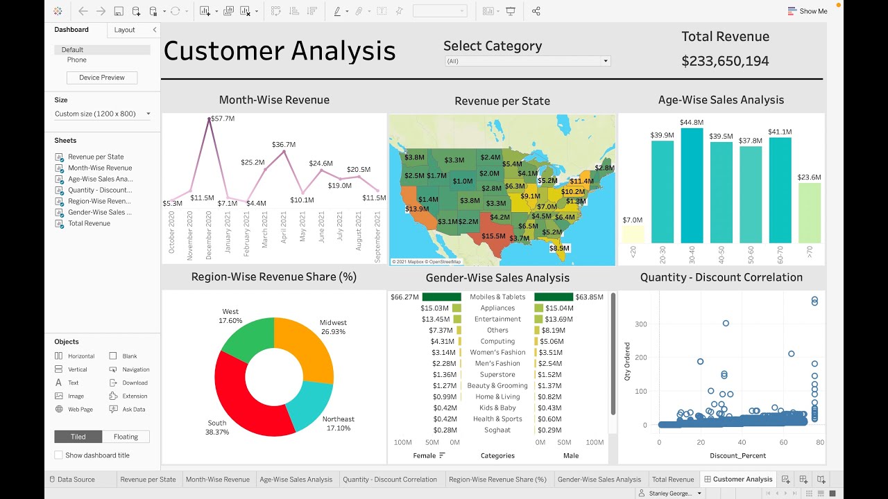
Customer Analysis using Tableau - Dashboard From Scratch

Full Project in Excel | Excel Tutorials for Beginners
Amazing‼️ Aplikasi Sistem Informasi Puskesmas Siap Pakai. Bisa Langsung Hosting
5.0 / 5 (0 votes)