Sampling Distributions: Introduction to the Concept

jbstatistics
28 Dec 201207:51

Summary

TLDRThis video script introduces the concept of sampling distributions, essential for statistical inference. It explains that the sampling distribution of a statistic, such as the sample mean, is the probability distribution of that statistic if samples were drawn repeatedly from a population. Using a university class example, the script illustrates how the sample mean varies across different samples and how this variation can be visualized through a histogram, approximating the true sampling distribution. The significance of understanding sampling distributions is highlighted for making statistical inferences about population parameters.

Takeaways

  • πŸ“š The concept of sampling distributions is fundamental to statistical inference techniques.
  • πŸ” A sampling distribution represents the probability distribution of a statistic based on repeated sampling from a population.
  • πŸ‘¨β€πŸ« The example of a university class with 16 students illustrates the concept, where the average age is the population parameter.
  • πŸ”’ The true population mean (mu) is an unknown quantity to the professor and is calculated as 239.8125 in the example.
  • 🎯 The professor uses a random sample of three students' ages to estimate the unknown population mean (mu).
  • πŸ“‰ The sample mean is calculated by averaging the ages of the sampled students, providing a point estimate for mu.
  • βš–οΈ The uncertainty of the sample mean as an estimate for mu is addressed using the sampling distribution of the sample mean.
  • πŸ“ˆ The histogram of sample means, obtained from repeated sampling, closely resembles the true sampling distribution of the sample mean.
  • πŸ“Š The sample mean is often distributed approximately normally, which is a common assumption in many statistical analyses.
  • πŸ€” The sampling distribution helps in understanding the variability of a statistic and its potential closeness to the true population parameter.
  • πŸ“ Mathematical arguments based on the sampling distribution are used to make inferences about population parameters, such as confidence intervals.

Q & A

  • What is the concept of a sampling distribution?

    -A sampling distribution is the probability distribution of a given statistic, showing how that statistic would vary if numerous samples of the same size were drawn from the population.

  • Why is the concept of a sampling distribution important in statistical inference?

    -The concept of a sampling distribution is crucial in statistical inference because it allows us to make inferences about population parameters based on the distribution of a statistic from multiple samples.

  • What is the difference between a population parameter and a sample statistic?

    -A population parameter is a numerical characteristic of the entire population, such as the population mean (mu). A sample statistic is an estimate of the population parameter derived from a sample, like the sample mean (X bar).

  • In the script, what is the example used to illustrate the concept of a sampling distribution?

    -The script uses the example of a university class with 16 students where the professor wants to know the average age of the students. The professor can only access the ages of a random sample of three students at a time.

  • How is the true population mean calculated in the script's example?

    -The true population mean (mu) is calculated by taking the average of the ages of all 16 students, which is given as 239.8125 in the script.

  • What is the purpose of drawing multiple samples in the script's example?

    -Drawing multiple samples serves to illustrate that the sample mean (X bar) will vary from sample to sample, highlighting the concept of the sampling distribution of the sample mean.

  • How is the sample mean calculated from a sample of students' ages?

    -The sample mean is calculated by summing the ages of the students in the sample and then dividing by the number of students in that sample.

  • What does the script suggest about the distribution of the sample mean in many situations?

    -The script suggests that in many situations, the distribution of the sample mean is approximately normal, even though the example provided does not show this.

  • How many possible samples are there in the script's example if the sample size is 3 and the population size is 16?

    -There are 560 possible samples when the sample size is 3 and the population size is 16, calculated using the combination formula 'n choose k' (16 choose 3).

  • What is the significance of the histogram of sample means in the script's repeated sampling argument?

    -The histogram of sample means represents the distribution of the sample mean across many repeated samples, providing an approximation of the true sampling distribution of the sample mean.

  • How does the concept of a sampling distribution help in making statements about population parameters?

    -The concept of a sampling distribution allows us to make probabilistic statements about population parameters, such as expressing confidence intervals for estimates of the population mean.

Outlines

00:00

πŸ“š Introduction to Sampling Distributions

This paragraph introduces the fundamental concept of sampling distributions in statistical inference. It explains that the sampling distribution of a statistic is its probability distribution when samples are repeatedly drawn from a population. The paragraph uses an example of a university class with 16 students to illustrate how the average age (a parameter) can be estimated through sampling. It highlights the variability of the sample mean (X bar) across different samples and emphasizes the importance of understanding the sampling distribution to estimate population parameters and quantify uncertainty.

05:02

πŸ“ˆ Understanding the Sample Mean's Distribution

The second paragraph delves deeper into the concept of the sample mean's distribution, focusing on how it is derived from the sampling distribution. It uses the same university class example to demonstrate that the sample mean is likely to vary with each sample drawn, and that this variability can be visualized through a histogram of sample means. The paragraph clarifies that while the sample mean's distribution is not always normal, it often approximates a normal distribution in many situations. It also explains that the histogram, which could be derived from a large number of repeated samples or calculated from all possible samples, closely resembles the true sampling distribution of the sample mean. The importance of this concept in statistical inference is underscored, as it allows for making probabilistic statements about population parameters.

Mindmap

Keywords

πŸ’‘Sampling Distribution

The sampling distribution refers to the probability distribution of a given statistic based on a random sample. It is central to the video's theme as it illustrates how the distribution of a statistic, such as the sample mean, would look if samples were taken repeatedly from a population. The script uses the concept to explain how the sample mean varies with each sample, and how this variation is crucial for statistical inference.

πŸ’‘Statistical Inference

Statistical inference is the process of making predictions or decisions about a population based on data from a sample. The video discusses this concept as it is the foundation for understanding how the sampling distribution of a statistic can be used to make inferences about the population parameters. The script mentions statistical inference as the broader application of the sampling distribution concept.

πŸ’‘Parameter

In statistics, a parameter is a numerical characteristic of a population that we are interested in estimating or testing. The video script introduces the concept by referring to 'mu' as the true average age of the students, which is a parameter that the professor is trying to estimate using the sample mean.

πŸ’‘Sample Mean

The sample mean, denoted as X bar in the script, is the average of the values in a sample. It is a key concept in the video as it is used to estimate the population mean. The script illustrates how different samples can yield different sample means, highlighting the variability inherent in the sampling process.

πŸ’‘Population Mean

The population mean, represented by 'mu' in the script, is the average of all values in the population. It is an important concept because it is the value that the sample mean is used to estimate. The script explains that the true population mean is unknown to the professor and must be inferred from the sample data.

πŸ’‘Random Sample

A random sample is a subset of a population in which each member of the subset has an equal chance of being selected. The script uses the concept of a random sample to demonstrate how the professor selects students to estimate the average age, emphasizing the importance of randomness in obtaining a representative sample.

πŸ’‘Histogram

A histogram is a graphical representation of the distribution of data, showing the frequency of data points within certain ranges or 'bins'. In the video, a histogram of sample means is used to visually represent the sampling distribution, illustrating the central tendency and dispersion of the sample means.

πŸ’‘Normal Distribution

The normal distribution, often referred to as a bell curve, is a probability distribution that is widely used in statistics. The script mentions that the sample mean often has a distribution that is approximately normal, which is important for making inferences about the population mean.

πŸ’‘Confidence Interval

A confidence interval is a range of values, derived from a sample, that is likely to contain the population parameter with a certain level of confidence. The script alludes to the concept by stating that we can make statements about how close the sample mean is likely to be to the true value of 'mu', which is the essence of a confidence interval.

πŸ’‘Estimation

Estimation in statistics involves using sample data to make an educated guess about a population parameter. The script discusses how the professor uses the sample mean to estimate the unknown population mean, which is a fundamental aspect of statistical inference.

πŸ’‘Variability

Variability refers to the extent to which data points differ from each other within a dataset. The script highlights variability by showing how different samples can yield different sample means, which is essential for understanding the sampling distribution and the uncertainty associated with estimates.

Highlights

The concept of sampling distributions is fundamental to statistical inference techniques.

The sampling distribution of a statistic is its probability distribution when samples are repeatedly drawn from the population.

The example of a university class with 16 students illustrates the concept of a sampling distribution.

The true population mean (mu) is an unknown quantity to the professor.

The professor can take a sample of three students to estimate the average age.

The true ages of the 16 students are given, but the professor is unaware of them.

The true population mean mu is calculated to be 239.8125, but it is unknown to the professor.

The professor draws a random sample of three students and calculates the sample mean.

The sample mean is used to estimate the unknown population mean mu.

The concept of uncertainty is introduced, questioning how close the sample mean is likely to be to the true mu.

Mathematical arguments based on the sampling distribution of the sample mean (X bar) are used to address uncertainty.

Repeated sampling shows that the sample mean will vary from sample to sample.

A computer simulation demonstrates the sampling distribution by repeatedly sampling a million times.

The histogram of sample means closely resembles the true sampling distribution of the sample mean.

The population mean mu is represented on the histogram with a red line.

The sample mean distribution is often approximately normal, as explained in later discussions.

The number of possible samples (16 choose 3) gives another perspective on the sampling distribution.

The histogram of sample means represents the distribution of all possible sample means of size 3 from the population.

In practice, only one sample is typically drawn, but the concept of a sampling distribution is crucial for statistical inference.

The sampling distribution allows making statements about population parameters with a certain level of confidence.

Transcripts

play00:02

Let's take a look at an introduction to the concept of sampling distributions.

play00:07

To a great extent, statistical inference techniques are based on the concept of

play00:11

the sampling distribution of a statistic.

play00:13

Later on we're going to be discussing statistical inference

play00:16

and so it is important that we get this notion of a sampling distribution down.

play00:22

The sampling distribution of a statistic is the probability distribution of that statistic.

play00:27

In other words it is the distribution of the statistic

play00:31

if we were to repeatedly draw samples from the population.

play00:34

So if we were to get a sample, get a value of a statistic,

play00:38

and draw different sample of the same sample size and get a value that statistic,

play00:42

the statistic is going to vary from sample to sample

play00:44

according to the sampling distribution of that statistic.

play00:52

Let's look at a simple example to illustrate.

play00:54

Suppose a university class has 16 students,

play00:57

and the professor wants to know the average age of the sixteen students in the class.

play01:01

Since the professor is interested in these specific 16 students,

play01:06

these 16 students represent the population of interest,

play01:09

and their average age is a parameter. And I'm going to call that mu.

play01:15

Perhaps the professor would have access to this information in their records

play01:18

but I'm going to assume here

play01:20

that they do not have access to this information,

play01:22

and so mu is an unknown quantity to the professor.

play01:27

I'm also going to assume in this bit of a contrived example that the professor

play01:30

can take a sample of three students and find out their ages.

play01:34

So perhaps it's something like the professor has a friend

play01:37

in the Registrar's Office who'll look up the ages of 3 students for them.

play01:40

Or something to that effect.

play01:43

Unknown to the professor, this is the reality of the situation.

play01:47

These are the true ages for the 16 students in the class.

play01:51

And this is the reality of the situation. We can calculate the true population mean mu.

play01:57

If we take the average of those 16 values,

play02:00

we would see that that is 239.8125.

play02:07

But that is an unknown value to the professor.

play02:12

To the professor, the reality of the situation looks something like this.

play02:16

There's 16 students with unknown ages.

play02:18

I'm going to number them so we can keep track of them.

play02:22

The professor is allowed to draw a random sample of three students and find out their ages.

play02:27

So let's randomly select three students.

play02:30

The red dots represent our randomly selected students,

play02:33

and we can find out their ages in months.

play02:35

We get ages of 233, 227, and 238.

play02:41

And we can calculate the sample mean of those three values simply by

play02:46

adding up those values and dividing by 3.

play02:50

And we get a value of the sample mean of 232.67,

play02:56

when rounded to two decimal places.

play03:00

We're going to use this value of the sample mean

play03:02

to estimate mu, which is an unknown quantity to the professor.

play03:09

In addition to this single value,

play03:11

this point estimate, that estimates mu.

play03:15

We would like to give some measure of the uncertainty associated with that value.

play03:21

How close is that value likely to be to the true value of mu?

play03:28

To answer that question

play03:30

we use mathematical arguments based on the sampling distribution of X bar.

play03:37

Related to that is the idea that if we were to draw another sample

play03:41

we would be very very unlikely to get this sample mean again.

play03:45

The sample mean is going to vary from sample to sample.

play03:49

Let's take a look at an example of that to illustrate.

play03:53

Here's our sixteen students again, and let's draw a random sample size 3.

play03:58

We get these three students and they have ages of 251, 238 and 276.

play04:04

And we can again calculate the sample mean of those values

play04:08

by simply adding them up and dividing by 3.

play04:12

And this time we get a sample mean of 255.

play04:19

And had we got this sample, we would use this value to estimate the unknown mu.

play04:26

Note that the sample mean we got here was different from

play04:29

the sample mean we got in our first sample.

play04:33

In repeated sampling the value of the sample mean would vary from sample to sample.

play04:39

The value of statistics vary from sample to sample.

play04:45

If we sampled many times, we did it twice here,

play04:49

but I've sped up the process using a computer and done it a million times.

play04:52

We plotted those sample means in a histogram,

play04:55

it would look something like this.

play04:59

and because I've repeatedly sampled so many times,

play05:02

this histogram of sample means will very closely resemble

play05:07

the true sampling distribution of the sample mean in this scenario.

play05:12

For a little perspective I'm going to put in

play05:15

the population mean mu with a red line.

play05:18

That's what this red line represents,

play05:19

our value of mu, which is about 240.

play05:25

We can note that the sample mean will be distributed

play05:28

about the population mean in some way.

play05:32

As we'll learn later on, very often the sample mean has a distribution that is approximately normal.

play05:39

Doesn't look like that here, but in many situations

play05:42

the sample mean does have a distribution that is approximately normal.

play05:46

Here we sampled 3 people from 16

play05:50

and thus there were 16 choose 3 or 560 possible samples.

play05:55

So another perspective on the sampling distribution here,

play05:59

is that in this scenario, the sampling distribution of the sample mean

play06:03

is the distribution of the sample mean in all possible samples

play06:08

of size 3 from this population.

play06:11

Going back to our histogram of sample means,

play06:14

we didn't have to actually repeatedly sample from the population.

play06:17

We had 560 possible samples and so we could have worked out

play06:22

the exact sampling distribution of the sample mean in this scenario.

play06:26

But I wanted to illustrate the repeated sampling argument.

play06:29

And since we repeatedly sampled so many times,

play06:32

this histogram will very very closely resemble

play06:37

the true sampling distribution of X bar in this scenario.

play06:44

Note that in practice we don't repeatedly sample from the population,

play06:48

and we typically draw only one sample.

play06:50

But the concept of a sampling distribution is an important one.

play06:56

The value of a statistic that we see in our sample

play06:59

will be a random sample from that statistic's sampling distribution.

play07:06

Why are we even talking about this slightly abstract concept?

play07:10

Well we will use mathematical arguments based on the statistic's sampling distribution

play07:15

to make statements about population parameters.

play07:19

So this is going to play an important role in statistical inference.

play07:24

When all is said and done

play07:26

we'll end up making statements like we are 95% confident

play07:30

the sample mean lies within 22.1 units of mu.

play07:35

And we're going to be allowed to say things like

play07:37

95% and 22.1

play07:41

based on mathematical arguments related to the sampling distribution of the sample mean.

Rate This
β˜…
β˜…
β˜…
β˜…
β˜…

5.0 / 5 (0 votes)

Related Tags
Sampling DistributionStatistical InferenceProbabilityPopulation MeanSample MeanEstimationUncertaintyData AnalysisEducationalStatistical Concepts