Model Evaluation using Visualization #datascience #datascience #technology #subscribeformore

Summary

This video script delves into model evaluation through visualization techniques. It emphasizes the utility of regression plots for estimating variable relationships, highlighting correlation strength and direction. The script guides on plotting these using Seaborn's 'regplot' and 'residplot' functions, illustrating how residual plots can reveal linearity or non-linearity in data. It also touches on distribution plots for visualizing models with multiple variables, showcasing how predicted and actual values compare, and how using multiple features can enhance model accuracy.

Takeaways

• 📈 Regression plots are essential for visualizing the relationship between two variables, indicating the correlation strength and direction.
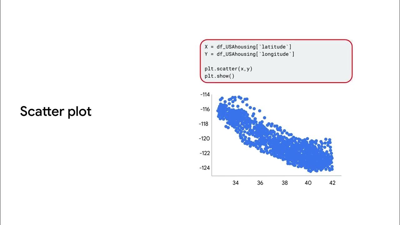
• 📊 The horizontal axis in a regression plot represents the independent variable, while the vertical axis represents the dependent variable.
• 📝 Each point in a regression plot corresponds to a different target, with the fitted line showing the predicted values.
• 🖋️ Seaborn's 'regplot' function is a simple method to create regression plots, requiring the column names for independent and dependent variables.
• 🔍 Residual plots help examine the error between predicted and actual values, providing insights into the model's fit.
• 📉 A residual plot with zero mean and evenly distributed values around the x-axis suggests a well-fitted linear model.
• 🌀 Curvature in a residual plot indicates that a non-linear function might be more appropriate for the data.
• 📊 Seaborn's 'residplot' function is used to create residual plots, showing the relationship between predicted and actual values.
• 📈 Distribution plots are useful for visualizing models with multiple independent variables, comparing predicted and actual values.
• 📊 In a distribution plot, the vertical axis is scaled to normalize the area under the distribution, useful for continuous values.
• 💡 The script illustrates the use of different visualization techniques to evaluate and understand the performance of regression models.

Q & A

What is the purpose of using regression plots in model evaluation?

Regression plots are used to estimate the relationship between two variables, determine the strength of the correlation, and identify the direction of the relationship (positive or negative).

What do the horizontal and vertical axes represent in a regression plot?

The horizontal axis represents the independent variable, while the vertical axis represents the dependent variable.

How is a regression plot created using the Seaborn library in Python?

First, import the Seaborn library. Then use the 'regplot' function, specifying the 'x' parameter for the independent variable, the 'y' parameter for the dependent variable, and the 'data' parameter for the dataframe containing the data.

What does a residual plot represent?

A residual plot represents the error between the actual value and the predicted value. It is plotted with the independent variable on the horizontal axis and the residuals (errors) on the vertical axis.

What does it indicate if the residuals are distributed evenly around the x-axis with similar variance?

If the residuals are evenly distributed around the x-axis with similar variance and zero mean, it suggests that a linear model is appropriate for the data.

What might it indicate if there is curvature in the residual plot?

Curvature in the residual plot indicates that the linear assumption may be incorrect, and a non-linear model might be more appropriate.

How can Seaborn be used to create a residual plot?

First, import the Seaborn library. Then use the 'residplot' function, specifying the independent variable series as the first parameter and the dependent variable series as the second parameter.

What is the purpose of a distribution plot in model evaluation?

A distribution plot is used to compare the predicted values to the actual values, helping visualize the accuracy of the model's predictions across a range of values.

How are continuous target values handled when creating a distribution plot using Pandas?

Since a histogram is for discrete values, Pandas converts continuous target values to a distribution, scaling the vertical axis to make the area under the distribution equal to one.

What does a distribution plot with the predicted and actual values reveal about the model's performance?

The distribution plot shows how close the predicted values are to the actual values. For example, in the provided script, predicted values for prices ranging from $10,000 to $20,000 are closer to the actual target values compared to the predicted values for prices ranging from $40,000 to $50,000.

Outlines

00:00

📊 Regression Plots for Model Evaluation

This paragraph discusses the use of regression plots to evaluate the relationship between variables in a model. It explains the significance of the horizontal and vertical axes, representing the independent and dependent variables respectively, and how each point on the plot signifies a different target point. The paragraph also introduces the concept of the fitted line, which indicates the predicted value. It further elaborates on how to create a regression plot using the seaborn library in Python, with specific parameters for the independent variable, dependent variable, and data frame. The importance of residual plots is highlighted as a tool to examine the error between predicted and actual values, with insights into how to interpret different patterns in these plots, such as zero mean distribution, curvature, and variance increase with the independent variable.

Keywords

💡Model Evaluation

Model evaluation is the process of assessing the performance of a predictive model. In the context of the video, it refers to using visualization techniques to understand the relationship between the model's predictions and the actual outcomes. The script discusses using regression plots and residual plots to evaluate the model's accuracy and the appropriateness of the linear assumption.

💡Regression Plots

A regression plot is a graphical representation that shows the relationship between the independent variable (on the horizontal axis) and the dependent variable (on the vertical axis). The script explains that each point in the plot represents a different target, and the fitted line represents the predicted values. Regression plots are essential for estimating the strength and direction of the correlation.

💡Correlation

Correlation measures the extent to which two variables are linearly related. The script mentions that regression plots help in estimating the strength of the correlation, which can be positive (both variables increase together) or negative (one variable increases as the other decreases). This concept is crucial for understanding the predictive power of the model.

💡Residual Plot

A residual plot is used to visualize the differences between the actual values and the predicted values of a model. In the script, it is explained that these plots can reveal if the errors are randomly distributed, which would suggest a good fit, or if there is a pattern, indicating a poor fit or the need for a non-linear model.

💡Seaborn Library

Seaborn is a Python visualization library based on matplotlib that provides a high-level interface for drawing attractive and informative statistical graphics. The script describes using Seaborn's 'regplot' and 'residplot' functions to create regression and residual plots, respectively, which are vital for model evaluation.

💡Independent Variable

An independent variable is a factor that is believed to influence the dependent variable in an experiment or study. In the script, the 'x' parameter in the 'regplot' function is used to represent the independent variable, which is crucial for plotting the relationship with the dependent variable.

💡Dependent Variable

A dependent variable is the outcome that is being measured or tested in an experiment. In the context of the script, the 'y' parameter in the 'regplot' function represents the dependent variable, which is the target value that the model is trying to predict.

💡Fitted Line

The fitted line in a regression plot is the line that best fits the data points according to the model's predictions. The script mentions that this line represents the predicted values and is a key element in evaluating how well the model is performing.

💡Residual Errors

Residual errors are the differences between the actual values and the predicted values from a model. The script discusses how examining these errors in a residual plot can provide insights into the model's performance and whether the assumptions of linearity are valid.

💡Distribution Plot

A distribution plot is used to visualize the distribution of data points. The script uses this concept to compare predicted values against actual values, particularly in the context of models with multiple features. It helps in understanding the accuracy of the model across different ranges of values.

💡Multiple Features

Multiple features refer to the use of more than one independent variable in a model. The script provides an example where using multiple features improves the model's predictions, bringing them closer to the actual target values, demonstrating the importance of considering various factors in model building.

Highlights

The video discusses model evaluation using visualization techniques.

Regression plots are used to estimate the relationship between variables and determine the strength and direction of correlation.

The independent variable is represented on the horizontal axis, and the dependent variable on the vertical axis in a regression plot.

Each point in a regression plot represents a different target, and the fitted line shows the predicted value.

Seaborn's regplot function can be used to create a regression plot with parameters for independent and dependent variables.

Residual plots represent the error between actual and predicted values.

A residual plot with zero mean and evenly distributed values suggests a linear relationship is appropriate.

Curvature in a residual plot indicates a non-linear relationship and the need for a non-linear function.

Seaborn's residplot function is used to create residual plots for further analysis.

Variance of residuals increasing with the independent variable suggests model inadequacy.

Distribution plots are useful for visualizing models with multiple independent variables.

A distribution plot compares predicted values against actual values, useful for continuous variables.

Predicted values are visualized in blue, and actual values in red within a distribution plot.

Distribution plots can reveal inaccuracies in predicted values for specific ranges.

Using multiple features improves the accuracy of predicted values compared to using a single feature.

The code for creating a distribution plot is provided, including parameters for actual and predicted values.

The video concludes with the importance of visualizing model predictions for accurate evaluation.

Transcripts

in this video we'll look at model

evaluation using visualization

regression plots are a good estimate of

the relationship between two variables

the strength of the correlation and the

direction of the relationship positive

or negative

the horizontal axis is the independent

variable

the vertical axis is the dependent

variable

each point represents a different target

point the fitted line represents the

predicted value

there are several ways to plot a

regression plot a simple way is to use

reg plot from the seaborne library

first import seaborn

then use the reg plot function the

parameter x is the name of the column

that contains the independent variable

or feature

the parameter y contains the name of the

column that contains the name of the

dependent variable or target the

parameter data is the name of the data

frame

the result is given by the plot

the residual plot represents the error

between the actual value

examining the predicted value and actual

value we see a difference

we obtained that value by subtracting

the predicted value and the actual

target value

we then plot that value on the vertical

axis with an independent variable as the

horizontal axis similarly

for the second sample we repeat the

process

subtracting the target value from the

predicted value

then plotting the value accordingly

looking at the plot gives us some

insight into our data

we expect to see the results to have

zero mean distributed evenly around the

x-axis with similar variance there is no

curvature

this type of residual plot suggests a

linear plot is appropriate

in this residual plot there is a

curvature

the values of the error change with x

for example in the region all the

residual errors are positive

in this area the residuals are negative

in the final location the error is large

the residuals are not randomly separated

this suggests the linear assumption is

incorrect

this plot suggests a non-linear function

we will deal with this in the next

section

in this plot we see that variance of the

residuals increases with x therefore our

model is incorrect

we can use seaborn to create a residual

plot

first import seaborn

we use the resid plot function

the first parameter is a series of

dependent variable or feature

the second parameter is a series of

dependent variable or target

we see in this case the residuals have a

curvature

a distribution plot counts the predicted

value versus the actual value

these plots are extremely useful for

visualizing models with more than one

independent variable or feature

let's look at a simplified example

we examine the vertical axis

we then count and plot the number of

predicted points that are approximately

equal to one

we then count and plot the number of

predicted points that are approximately

equal to two

we repeat the process for predicted

points they're approximately equal to

three

then we repeat the process for the

target values

in this case all the target values are

approximately equal to two

the values of the targets and predicted

values are continuous

a histogram is for discrete values

therefore pandas

will convert them to a distribution

the vertical axis is scaled to make the

area under the distribution equal to one

this is an example of using a

distribution plot the dependent variable

or feature is price the fitted values

that result from the model are in blue

the actual values are in red

we see the predicted values for prices

in the range from forty thousand to

fifty thousand are inaccurate

the prices in the region from ten

thousand to twenty thousand are much

closer to the target value in this

example we use multiple features or

independent variables

comparing it to the plot on the last

slide

we see predicted values are much closer

to the target values

here is the code to create a

distribution plot

the actual values are used as a

parameter

we want a distribution instead of a

histogram so we want the hist parameter

set to false

the color is red the label is also

included

the predicted values are included for

the second plot the rest of the

parameters are set accordingly

[Music]