Normal Approximation to Sample Mean

Summary

This video explains the Central Limit Theorem (CLT) and its applications in statistical inference. The speaker demonstrates how the sample mean (X̄) is an unbiased estimate of the population mean (μ), and how CLT ensures that for large sample sizes, the distribution of X̄ approximates a normal distribution. The video uses simulations to show how increasing sample size improves the approximation and discusses the concept of confidence intervals, which quantify the probability that the population mean lies within a specific range. The CLT is highlighted as a powerful tool in estimating and making predictions about larger populations.

Takeaways

• 😀 The sample mean (X̄) is an unbiased estimate of the population mean (μ).
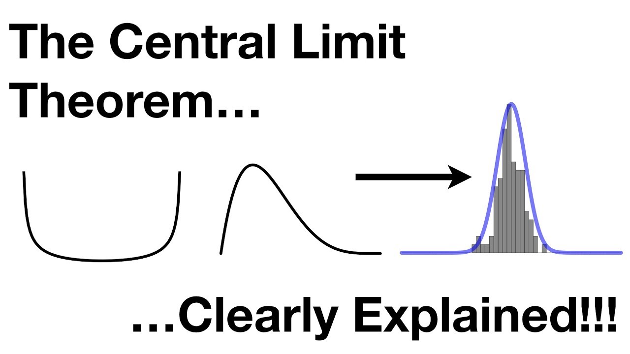
• 😀 According to the Central Limit Theorem (CLT), the distribution of the sample mean becomes approximately normal as the sample size increases.
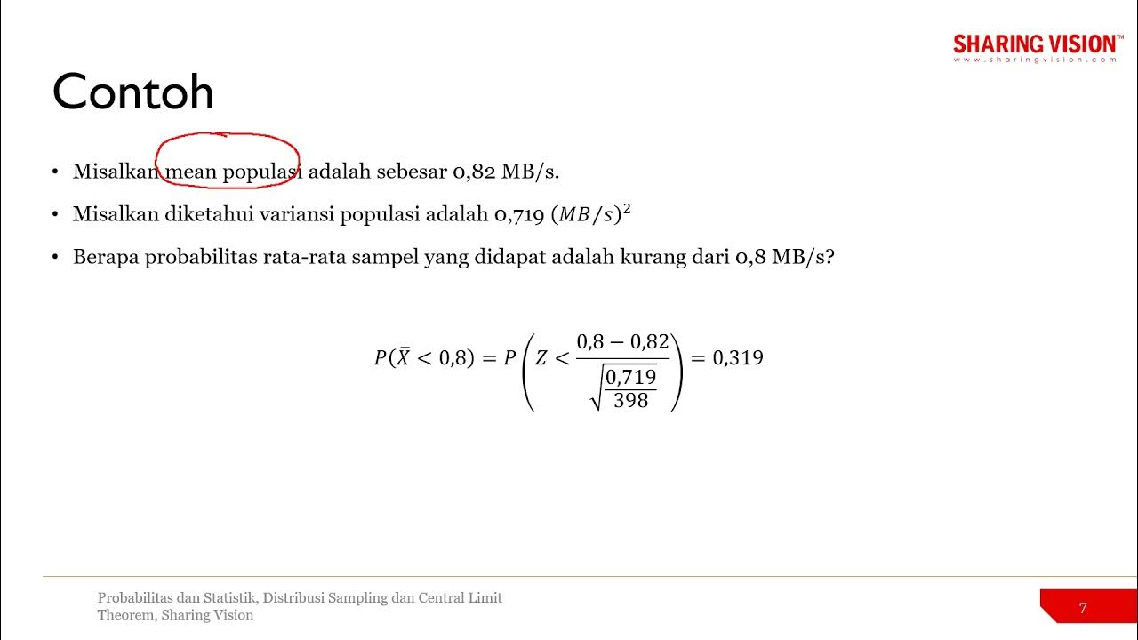
• 😀 The sample mean (X̄) has a mean of μ and a standard deviation (standard error) of σ/√n, where σ is the population standard deviation and n is the sample size.
• 😀 The Central Limit Theorem allows for precise statistical statements about the sample mean, even when the population distribution is not normal.
• 😀 To apply the Central Limit Theorem effectively, a sample size of at least 30 is typically sufficient for the sample mean to approximate normality.
• 😀 By generating random samples and computing their means, we can observe the normal distribution of the sample mean, as predicted by CLT.
• 😀 Increasing the sample size (n) results in a more accurate approximation of the normal distribution for the sample mean (X̄).
• 😀 Confidence intervals can be calculated by normalizing the sample mean and using the cumulative distribution function (CDF) of the standard normal distribution.
• 😀 The probability that the sample mean is within a specified tolerance (ε) of the population mean can be calculated using standard normal properties.
• 😀 The standard error (σ/√n) quantifies the variability of the sample mean, and increasing sample size reduces this variability, improving the accuracy of estimates.

Q & A

What is the Central Limit Theorem (CLT)?

The Central Limit Theorem states that the sampling distribution of the sample mean will approach a normal distribution as the sample size increases, regardless of the shape of the population distribution. This normal distribution has the same mean as the population but a smaller variance, specifically σ²/n, where σ² is the population variance and n is the sample size.

How does the sample mean relate to the population mean?

The sample mean (x̄) is an unbiased estimator of the population mean (μ), meaning that the expected value of the sample mean equals the population mean. This allows the sample mean to be used as a reliable estimate of the population mean in statistical analysis.

What is the significance of the standard error in relation to the sample mean?

The standard error is the standard deviation of the sample mean distribution, given by σ/√n, where σ is the population standard deviation and n is the sample size. It indicates how much the sample mean (x̄) is expected to vary from the population mean (μ). A smaller standard error means more precise estimates of the population mean.

Why is the sample size important when using the Central Limit Theorem?

The sample size is important because the Central Limit Theorem states that the distribution of the sample mean becomes more normal as the sample size increases. A sample size of at least 30 is generally considered sufficient for the CLT to apply. Larger sample sizes result in a more accurate normal approximation and smaller standard errors.

What is a confidence interval, and how is it related to the CLT?

A confidence interval is a range of values within which the true population mean (μ) is likely to lie, based on the sample mean (x̄) and the standard error. The Central Limit Theorem allows us to estimate this range by using the normal distribution, where the sample mean follows a normal distribution with mean μ and standard deviation σ/√n.

How does the code simulation in the transcript demonstrate the Central Limit Theorem?

The code simulation demonstrates the CLT by repeatedly taking random samples from a large population and calculating the sample mean for each. The histogram of these sample means is plotted, and as the sample size increases, the distribution of the sample mean becomes more normal, closely matching the predicted normal distribution from the CLT.

What happens when the sample size is increased in the simulation?

When the sample size is increased in the simulation, the approximation to a normal distribution becomes more accurate. This is because larger sample sizes reduce the standard error, making the sample mean distribution closer to the population mean and the normal distribution predicted by the CLT.

What is the role of the standard normal distribution in the CLT?

The standard normal distribution is used to normalize the sample mean (x̄). By subtracting the population mean (μ) and dividing by the standard error (σ/√n), we standardize the sample mean to follow a normal distribution with a mean of 0 and a standard deviation of 1. This allows for easier computation of probabilities and confidence intervals.

How do we calculate the probability that the error in the sample mean is within a certain tolerance?

To calculate the probability that the error (x̄ - μ) is within a certain tolerance (ε), we first normalize the error by dividing by the standard error (σ/√n). This gives a Z-score, which follows a standard normal distribution. We can then use the cumulative distribution function (CDF) of the standard normal distribution to compute the probability that the error is within ±ε.

Why is the sample variance (σ²) important when using the CLT and calculating confidence intervals?

The sample variance (σ²) is important because it is used to calculate the standard error, which in turn is used in the Central Limit Theorem and confidence intervals. A higher variance results in a larger standard error, leading to less precise estimates of the population mean. The more accurate the estimate of σ², the more reliable the confidence interval will be.