Elementary flows [Aerodynamics #9]

Summary

This lecture delves into incompressible and inviscid aerodynamics, focusing on irrotational flows and Bernoulli's equation. It introduces elementary flows as building blocks for complex aerodynamic analyses, covering uniform flow, source/sink, doublet, and vortex. The script explains how to construct these flows analytically using stream functions and velocity potentials, and demonstrates creating aerodynamic flow fields for bodies like the semi-infinite body, Rankine oval, stationary, and rotating cylinders. It concludes with practical applications in computational fluid dynamics, highlighting source and vortex panel methods.

Takeaways

• 📚 The lecture focuses on incompressible and inviscid flows, introducing the Bernoulli equation and the Laplace equation for velocity potential and stream function.
• 🌀 The concept of irrotationality allows for the application of Bernoulli's equation universally if the flow is irrotational, and both velocity potential and stream function satisfy the Laplace equation.
• 🏗️ Elementary flows are the building blocks of aerodynamics, including the uniform flow, source and sink, doublet, and vortex, which can be combined to model more complex flows.
• 🔍 The Laplace equation's linearity allows for the superposition of solutions, meaning different elemental flows can be added together to describe more complex flow patterns.
• 💡 Inviscid flow does not have boundary layers, eliminating the no-slip condition and allowing fluid to move freely without viscosity affecting its motion.
• 📐 Cylindrical coordinates are used predominantly in the lecture due to the round nature of many elementary flows, making it a more natural choice than Cartesian coordinates.
• 🌊 The uniform flow represents translational movement and is a fundamental component in constructing other flow models.
• 💧 Sources and sinks are opposite flows characterized by streamlines that emit outwards or inwards from a single point, with their strength defined by the volumetric flow rate per unit span.
• 🔗 The doublet is formed by combining a source and a sink very close together, with its strength defined by the constant product of lambda and the separation distance as the distance approaches zero.
• 🌀 The vortex flow is characterized by fluid orbiting a central point, with no radial velocity and a constant angular velocity, and its strength is defined by circulation.
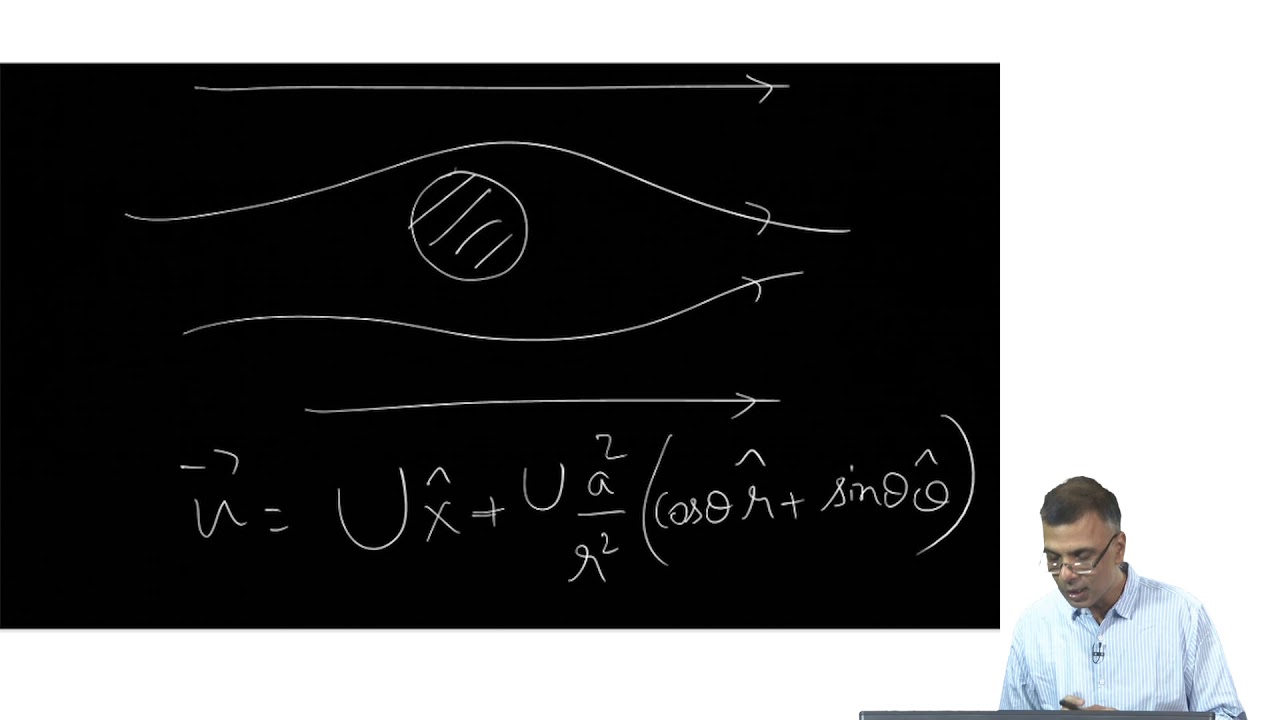
• 🛠️ The lecture demonstrates constructing more complex flows such as the semi-infinite body, Rankine oval, stationary cylinder, and rotating cylinder using the elemental flows as building blocks.
• 🔧 Computational Fluid Dynamics (CFD) commonly utilizes these elementary flows in flow-solving techniques, such as source panel and vortex panel methods for modeling flow around bodies.

Q & A

What are the two main equations in the field of incompressible and inviscid flows?

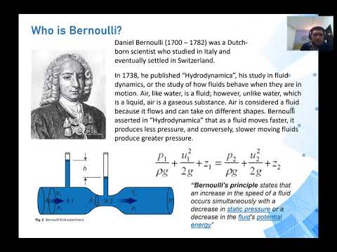
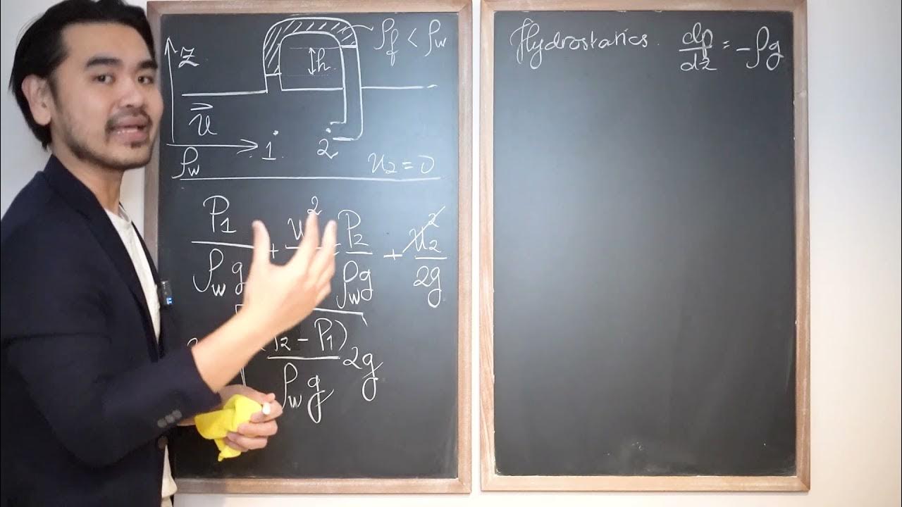
The two main equations are the Bernoulli equation, which relates pressure and velocity along a streamline, and the Laplace equation, which is satisfied by both the velocity potential and the stream function if the flow is irrotational.

Why is the Bernoulli equation applicable everywhere if the flow is irrotational?

The Bernoulli equation is applicable everywhere in an irrotational flow because the flow's properties can be described by a velocity potential, which is a scalar quantity that satisfies the Laplace equation, allowing for the conservation of mechanical energy along a streamline.

What is the significance of being able to add solutions of the Laplace equation together?

The ability to add solutions of the Laplace equation together is significant because it allows for the creation of complex flow fields by superimposing multiple elemental flows, each with its own stream function and velocity potential.

What are the four main elementary flows covered in the lecture?

The four main elementary flows are the uniform flow, the source and sink, the doublet, and the vortex.

How does the absence of boundary layers in inviscid flow affect the fluid movement over surfaces?

In inviscid flow, the absence of boundary layers means that there is no viscosity to slow down the fluid, and there is no no-slip condition to consider, allowing the fluid to move freely over surfaces.

What is the definition of a source and sink in the context of elementary flows?

A source and sink are elementary flows characterized by streamlines that emit outwards (source) or inwards (sink) from a single point. They are identical in nature but opposite in direction, with the source having a positive volumetric flow rate and the sink having a negative one.

How is the stream function for a source or sink constructed in cylindrical coordinates?

The stream function for a source or sink in cylindrical coordinates is constructed by using the radial velocity, which is the volumetric flow rate divided by the local circumference (2πr), and setting the azimuthal velocity to zero. The stream function is then expressed as a function of r and θ, with the sign depending on whether it is a source or sink.

What is the concept of a doublet in elementary flows, and how is it created?

A doublet is created by combining a source and a sink with equal and opposite strengths that are placed very close together. As the distance between them approaches zero and the product of the distance and the flow rate remains constant, the doublet is formed, characterized by a strength parameter k or kappa.

How is the vortex flow characterized in terms of its velocity field?

The vortex flow is characterized by having no radial velocity and a constant angular velocity, defined by the circulation divided by 2π. It represents fluid orbiting around a central point, with the flow being irrotational everywhere except at the center.

What is the practical application of elementary flows in computational fluid dynamics (CFD)?

In CFD, elementary flows are commonly used in flow solving techniques such as the source panel method for non-lifting bodies and the vortex panel method for lifting bodies. These methods involve defining the surface of a body as a series of sources or vortices and using stream functions to recreate the boundary of the body.

Outlines

00:00

📚 Introduction to Incompressible and Inviscid Flows

The lecture delves into the principles of incompressible and inviscid flows, highlighting the significance of irrotationality in these fluid dynamics scenarios. The Bernoulli equation is introduced, which links pressure and velocity in rotational flow, and is universally applicable if the flow is irrotational. The lecture also revisits the Laplace equation, satisfied by both the velocity potential and the stream function in irrotational flow, and emphasizes the additive property of solutions to these equations, allowing for the creation of complex flow patterns by superimposing elemental flows. The absence of boundary layers in inviscid flow is noted, which facilitates the analysis of aerodynamic objects using streamlines and flow fields.

05:01

🌀 Exploring Elementary Flows in Aerodynamics

This section focuses on elementary flows, which are fundamental components in aerodynamics, serving as building blocks for more complex flow patterns. The four primary elementary flows discussed are uniform flow, source and sink, doublet, and vortex. The uniform flow represents a constant velocity field, while the source and sink describe radial flow emanating from or converging towards a point. The doublet is a combination of a source and sink in close proximity, and the vortex involves fluid circulating around a central point. Each flow is examined in terms of its velocity field, stream function, and velocity potential, primarily using cylindrical coordinates due to the round nature of many elementary flows.

10:02

🛠 Constructing Complex Flows from Elementary Components

The script outlines the process of constructing more intricate aerodynamic flows by combining elementary flows. It begins with the semi-infinite body, which is formed by combining a uniform flow and a source. The Rankine oval is created by adding a uniform flow, a source, and a sink of equal strengths. The stationary cylinder flow is generated by summing a uniform flow and a doublet, while the rotating cylinder flow incorporates a vortex into the stationary cylinder flow. Each constructed flow is analyzed for stagnation points, which are crucial for defining the body's boundary in inviscid flow. The importance of understanding these stagnation points and their impact on the flow field is emphasized.

15:04

🔍 Analyzing Stagnation Points and Streamlines in Flow Fields

This part of the script provides a detailed examination of stagnation points and streamlines within the constructed flow fields. For the semi-infinite body, the stagnation point is identified at a specific radial distance and angle from the origin, defined by the center of the source. The Rankine oval's stagnation points are determined to be at the upstream and downstream tips of the oval shape. The stationary cylinder's stagnation points are located on the cylinder's surface, while the rotating cylinder's stagnation points can shift off the cylinder surface depending on the circulation strength. The analysis illustrates the dynamic nature of stagnation points and their significance in defining the flow around bodies.

20:05

🚀 Practical Applications of Elementary Flows in Aerodynamics

The final section of the script connects the theoretical concepts of elementary flows to practical applications in computational fluid dynamics (CFD). It mentions the source panel method for non-lifting bodies and the vortex panel method for lifting bodies, both of which utilize elementary flows to model complex flow scenarios around aerodynamic shapes. The script concludes with a review of the key points covered in the lecture, including the linearity of potential and stream functions, the introduction of four elemental flows, and the construction of complex flows representative of those around bodies.

Keywords

💡Aerodynamics

Aerodynamics is the study of the motion of air and other gases relative to solid objects, such as wings and bodies of aircraft. In the video, aerodynamics is the overarching theme as it discusses the principles and equations governing the flow of air around objects, which is crucial for understanding lift, drag, and stability in flight.

💡Incompressible Flow

Incompressible flow refers to a type of fluid flow where the density of the fluid does not change over time. In the context of the video, incompressible flow is an assumption used to simplify the analysis of fluid dynamics, allowing for the use of certain equations like the Bernoulli equation without considering changes in fluid density.

💡Inviscid Flow

Inviscid flow is a theoretical flow where the fluid has no viscosity, meaning it does not experience internal friction. The video script discusses inviscid flows to illustrate idealized fluid behavior without the complications of viscosity, which simplifies the mathematical modeling of fluid motion around objects.

💡Irrotational Flow

Irrotational flow is a type of flow where the fluid particles do not rotate about any axis. The video explains that if a flow is irrotational, the Bernoulli equation can be applied everywhere, and the velocity potential and stream function satisfy the Laplace equation, which is fundamental for analyzing elementary flows.

💡Bernoulli Equation

The Bernoulli equation is a fundamental principle in fluid dynamics that relates the pressure, kinetic energy, and potential energy per unit volume along a streamline in an inviscid, incompressible flow. In the video, it is mentioned as a key equation that works for rotational flow and is essential for understanding the relationship between pressure and velocity in a flow field.

💡Laplace Equation

The Laplace equation is a second-order partial differential equation that arises in various fields, including fluid dynamics. In the context of the video, the Laplace equation is satisfied by the velocity potential and stream function for incompressible, irrotational flows, which is crucial for constructing elementary flows.

💡Elementary Flows

Elementary flows are idealized flow patterns that represent basic building blocks in fluid dynamics. The video script delves into four main elementary flows: uniform flow, source and sink, doublet, and vortex. These flows are used to construct more complex flow patterns around aerodynamic bodies.

💡Stream Function

The stream function is a mathematical tool used in fluid dynamics to describe the flow of a fluid. It is particularly useful in two-dimensional flow analysis. In the video, the stream function is used to build the flow patterns for elementary flows and to represent the flow around objects by adding solutions of different elementary flows.

💡Velocity Potential

Velocity potential is another concept used in fluid dynamics to describe the flow field, particularly for incompressible and irrotational flows. It is related to the velocity field through the Laplace equation. The video explains how the velocity potential is constructed for different elementary flows and how it contributes to the overall flow field.

💡Uniform Flow

Uniform flow is a type of flow where the velocity is constant at every point in the flow field. In the video, uniform flow is described as having a constant stream-wise velocity and a zero vertical velocity, representing the translational movement of an object and serving as a fundamental component in constructing more complex flows.

💡Source and Sink

In fluid dynamics, a source and sink represent points where fluid emanates from or is absorbed into a surface, respectively. The video script explains these as elementary flows characterized by streamlines that emit outwards (source) or inwards (sink) from a single point, with their strength defined by the volumetric flow rate per unit span or depth.

💡Doublet

A doublet is a theoretical construct in fluid dynamics that results from combining a source and a sink very close together. The video describes the doublet as not being a unique building block because it is essentially a source and sink combined, with the strength of the doublet defined by the product of lambda and the separation distance as the distance approaches zero.

💡Vortex

A vortex, specifically a point vortex in the context of the video, is a flow where fluid particles orbit around a central point. The video explains that the vortex is characterized by having no radial velocity and a constant angular velocity, with the strength of the vortex defined by circulation, which is an important concept in the study of rotational flows.

💡Rankine Oval

The Rankine oval is a theoretical shape that results from the flow around an oval body, created by combining a uniform flow with a source and sink of equal and opposite strength. The video script uses the Rankine oval to illustrate how elementary flows can be combined to represent the flow around a closed body.

💡Stagnation Points

Stagnation points are locations in a flow field where the fluid velocity is zero. In the video, stagnation points are important for identifying the boundary of the flow around a body, as they often lie on the streamline that best represents the body's shape. The script discusses how to find stagnation points for various constructed flows, such as the semi-infinite body and the Rankine oval.

💡Computational Fluid Dynamics (CFD)

CFD is a branch of fluid mechanics that uses numerical methods and algorithms to solve and analyze problems involving fluid flows. The video mentions CFD in the context of how elementary flows are commonly used in CFD software, where they are built into the solvers to model complex flow scenarios around bodies.

Highlights

Introduction to incompressible and inviscid flows with irrotationality, leading to the Bernoulli equation and Laplace equation.

Exploration of the Bernoulli equation's application in rotational and irrotational flow scenarios.

Explanation of how velocity potential and stream function satisfy the Laplace equation for irrotational flow.

Discussion on the additive property of solutions to the Laplace equation, allowing for the combination of different flow features.

Insight into the absence of boundary layers in inviscid flow, eliminating the no-slip condition.

Introduction of elementary flows as building blocks for complex aerodynamic flows.

Description of the uniform flow and its representation of translational movement.

Explanation of source and sink flows, including their characteristics and the role of volumetric flow rate.

Introduction of the doublet flow, a combination of a source and sink in close proximity.

Derivation of the stream function and velocity potential for the doublet flow.

Introduction and characteristics of the vortex flow, including its irrotational nature except at the center.

Construction of complex flows using elementary flows, such as the semi-infinite body from a uniform flow and a source.

Identification of stagnation points in flow fields and their significance in body boundary representation.

Construction of the Rankine oval using a uniform flow, source, and sink.

Explanation of the stationary cylinder flow as a sum of a uniform flow and a doublet.

Introduction of the rotating cylinder flow by adding a vortex to the stationary cylinder flow.

Practical applications of elementary flows in computational fluid dynamics (CFD) and common flow solving techniques.

Discussion on source panel and vortex panel methods in CFD for non-lifting and lifting bodies, respectively.

Transcripts

hello and welcome to our ninth

lecture in aerodynamics last time

we started to explore specifically

incompressible and

inviscid flows with a hint of

irrotationality sprinkled throughout

this led us to two gigantic equations in

the field

the bernoulli equation which relates the

pressure and velocity along a streamline

for rotational flow

and if the flow is irrotational

bernoulli works everywhere

also if the flow is irrotational we

showed that both the velocity potential

and the stream function satisfy the

laplace equation

today we are going to continue our dive

into incompressible and

inviscid flows and start to look at

elementary flows

in a way these are small packages of

unique flow features that represent

building blocks for aerodynamics

the main four we will cover today are

the uniform flow

the source and sink the doublet

and the vortex

before we jump in let's recall some

things we've learned in the past

if flow is incompressible and

irrotational

we know that we can use the laplace

equation on the stream function

and the velocity potential these are

second order linear partial differential

equations

there are probably many important

features of these types of equations

but what's most important to us is that

that means we can add

solutions to these equations together

example if we want to recreate the flow

over an oval

which we will learn shortly we can

simply superimpose three separate

elemental flows by adding them together

we can add their stream functions and we

can add their velocity potentials

and in the end we have equations that

describe the oval

flow so let's remember that we can add

the solutions together

and we'll put this in the back of our

heads and call it a

now a useful feature of inviscid flow is

that we do not have boundary layers on

our surfaces

this means that the fluid can move

freely without viscosity slowing it down

and there's no longer a no-slip

condition to worry about

if we have an object we would like to

learn about aerodynamically

we can recreate that object shape and

streamlines

we can fully describe the flow field

over that object assuming flow is

irrotational

and that's really the point of today is

trying to make quote unquote

objects in a flow with streamlines using

building blocks

we're going to essentially build

aerodynamic flows from scratch

so let's jump right into the elementary

flows

elementary flows continue to fall under

our umbrella of inviscid

and incompressible flow meaning

viscosity is zero and density is

constant

these are the building blocks of

aerodynamic flows allowing us to create

complex flow fields completely

analytically

note today is mostly in cylindrical

coordinates

it's just unavoidable so many of our

elementary flows are round

so it makes more sense to use a polar

coordinate system than a cartesian one

there are four main basic flows that

we'll cover today

the uniform flow the source and sink

the doublet and the vortex we're going

to consider each individually

but build them in a way that they're

easy to compare to one another

we'll look at the velocity field the

stream function

and the velocity potential for each flow

the uniform flow

is just a constant velocity field where

the stream-wise velocity is a constant u

infinity

and the vertical velocity is zero we can

build the stream function from the

velocity field

by definition u is d

psi d y which is u infinity

v is d psi dx which is zero

using these two equations to solve for

psi

we can find the stream function in

cartesian coordinates

however the rest of our fields will be

in cylindrical coordinates

so let's transform it next up we have

the velocity potential

similarly we can build it from the

velocity field

using the definition of the velocity

potential

this leads us to the cartesian

definition of the velocity potential for

a uniform flow

which will turn into cylindrical

coordinates again

this elemental flow represents

translational movement of an object and

will be the main

ingredient for almost all of our flows

next we have the source and the sink

which are identical flows but opposite

in direction

they are characterized by having

streamlines that emit outwards or

inwards along straight stream lines

coming from a single point

sources flow out and sinks suck in

the velocity field is characterized by

the volumetric flow rate per unit span

or depth represented by lambda if we're

working with a source

the volumetric flow rate is positive and

for a sink it's negative

note we're starting now with the

cylindrical coordinates outright

the radial velocity u sub r is the

volumetric flow rate divided by the

local circumference 2 pi r

the azimuthal velocity u theta is by

definition 0.

again we build the streamlines by

starting with the velocity field and

using the definition of the stream

function

in cylindrical coordinates this gives us

a simple expression for the source and

sync stream function

if it's a source this is positive and

it's if it's a sink this is negative

and finally we build the velocity

potential from the velocity field using

its defined equations

next we move on to the doublet the

doublet is not a unique building block

because it's really just a source and a

sink combined and shoved really close

together consider a source in sync

both with equal and opposite strengths

separated by the distance l

what we do to make a doublet is shrink l

to 0

while simultaneously keeping the

parameter l

times lambda a constant this means that

as

l goes to 0 lambda approaches infinity

this constant lambda l represents the

strength of the doublet

instead of building the stream function

from the velocity as we've done before

we can build it by putting a source and

sync stream function together

and taking it to these limits and

constraints

start by adding the stream function of a

source in sync with equal and opposite

strength

note here that each get their own theta

coordinate

let's define the difference between

theta one and theta two to be delta

theta and rewrite the equation

from trigonometry and the small angle

approximation

we can define delta theta into l sine

theta divided by r

this gives us our final form of the

stream function for a doublet in

cylindrical coordinates

now we'll define the velocity potential

from the stream function

essentially with one step we're going to

convert the stream function to the

velocity field and then the velocity

field to the

velocity potential this gives us two

equations for the velocity potential

with unknown functions of integration

these can be solved for the final form

of the velocity potential for a doublet

in cylindrical coordinates

you'll see the strength of the doublet l

times lambda which is a constant

called k or kappa in a lot of places

and now we move on to our final

elemental flow the vortex

this is characterized by having a fluid

orbiting around

some central point the flow field is

defined by having no radial velocity

and a constant angular velocity thus

constant c

over the radial coordinate an

interesting feature of this vortex

sometimes referred to as a point vortex

is that it is

irrotational everywhere except at the

center point

much like a ferris wheel the constant

that defines the azimuthal velocity

u theta is the circulation divided by 2

pi

the strength of the vortex is tuned via

this circulation

you might notice that each elemental

flow has a parameter to tune the

strength

the uniform flow has u infinity the

sources and sinks have lambda

the doublet has k or kappa which is

lambda times

l and the vortex has circulation

from the velocity field as we've done

before let's build the stream function

and finally let's build the velocity

potential from the velocity field

you might be wondering why do we bother

with all this

well now we can use these stream

functions and velocity potentials to

build complex flows

by adding them together

let's get started by building some

relatively simple flows from our

building blocks

today we'll cover the semi-infinite body

the rankine oval

the stationary cylinder and the rotating

cylinder

first up we have the semi-infinite body

which is what you get when you add

together a uniform flow

and a source you'll notice that the

final streamlines of our flow

take the shape of what looks like a body

what we'll do here for each flow that we

build is first to find the stream

function

and then velocity field if we can then

talk about the stagnation points and the

streamlines that conveniently represent

the body

from above we know the stream function

for a uniform flow

and a source separately adding them

together gives us the stream function

for this complex flow

let's mark this down as the final form

of the stream function for a

semi-infinite body

once we have the stream function we can

take spatial derivatives of it to get

the velocity field

keep in mind we're still using the

cylindrical coordinate system

so the cylindrical version of the stream

function definition is used

in these flows the stagnation points are

important

because they often lie on the streamline

that best represents a body's boundary

for that particular flow

looking above we can identify the

stagnation point

the streamline with the stagnation point

after splitting

looks a lot like the boundary that

represents our semi-infinite body

so we want to find our stagnation point

or

points in the flows when we build them

by definition stagnation has a zero

radial and

azimuthal velocity

let's write down our velocity field

again and determine from the two

equations where in the field both

equations are zero

the coordinate for stagnation and this

flow is at a theta angle of pi

or 180 degrees and a distance from the

origin of lambda over two pi

u infinity note here that the origin is

defined by the center of the source

now the streamline that has stagnation

point is found by taking the stream

function

and evaluating it at this coordinate

from above we know the stream function

sine of pi is zero so the entire first

term goes away

the second term simplifies and we get

that psi equals lambda over 2

and that's the constant that represents

the streamline with the boundary on it

using the streamline we can define the

flow outside of it to be equal to the

flow around a semi-infinite body

if it existed in our flow

next we consider our first closed body

the rankine oval

this is defined as a uniform flow plus a

source

and sink of equal and opposite strength

the resulting streamline field looks a

lot like flow around an

oval

here let's note the center of the source

and sink

and define the origin to be at the

center of our oval

the source and sink are both a distance

b away from the origin

now the fact that the source and sink

are off of the origin

will present some coordinate

difficulties for us pretty soon

consider some point in our flow the

origin

the source and the sink all have

different angles

and radial locations relative to this

point

it's important to keep this in mind

moving forward

first up we define the stream function

by adding the stream function of each

component individually

in our stream function theta 1 and theta

2

are the angles from the source and sinks

reference frames

since the source and sink are not at the

origin these theta 1

and theta 2 angles are functions of the

azimuthal and radial coordinate from the

true origin

theta and r and the distance of the

source in sync from the origin

b let's quickly sketch the system and

see if we can figure out theta 1 and

theta 2 with trigonometry

what we find is that these angles are

inverse tangent functions of the

origin's coordinates and b

now if we truly define the velocity

field

we need to incorporate these angle

functions into the stream function

in order to take accurate derivatives

and that would be pretty nasty lucky for

us

we rarely need the velocity field itself

and we can skip that here

if you ever did need it you could just

do it out with the derivatives as

defined

since we don't have the velocity field

to truly calculate our stagnation

locations

we have to do it by inspection

if our flow represents the flow around

an oval we can expect that the

stagnation will happen at the upstream

and downstream

tips of our body this means that

theta equals theta one equals theta two

which is at the angular coordinates of

zero and pi

which represent the back and front of

the oval respectively

knowing this we can plug it into our

stream function

equation and simplify the first term is

zero because the sine function for these

theta coordinates

is zero and the last two terms are

always equal and opposite when they have

shared theta values

or when theta one equals theta two

so we find that psi equals zero for the

stagnation points

this constant represents the streamline

that best

represents the body because it has the

stagnation points on it

so we set the original stream function

equation

equal to zero to define this streamline

now we move to a special flow where

essentially the source and sink are

merged

this is a flow over a stationary

cylinder and is the sum of a uniform

flow

and a doublet here we see that when we

add the streamlines of a doublet in

uniform flow

we get a stream pattern that represents

a two-dimensional circle

which is a cylinder when considered

extension in the third dimension

as we've done in the past add the stream

functions of the individual flows

together

to get the stream function of the

cylinder flow

let's do some convenient rearranging and

bundle some constants that we'll define

as being the square

of the circle radius

then we can rewrite our simplified

expression for the stream function

we get the velocity field by taking the

spatial derivatives of the stream

function

by now we're experts at estimating the

stagnation point locations which we can

see happens at the radial and azimuthal

coordinates r

and 0 and r and pi

notice that if we were to plug these

values into the stream function

for both cases the stream function would

equal 0.

this means that the constant 0

represents the streamline of the

cylindrical body

when the stream function is set equal to

that constant

everything outside of this boundary

stream line represents flow

over a stationary cylinder

and last we have our first opportunity

to use the vortex flow

if we take stationary cylinder flow and

add a vortex

we get the case of a rotating cylinder

adding rotation adds a lot of

interesting features to the flow

which we'll explore more later in our

studies but here we

will explore what it does to the

streamline field

with rotation we can see that it pulls

more of the streamlines up above the

cylinder

and less passes underneath

to define the stream function officially

we add the stationary cylinder case

to the vortex stream function

note here the vortex cylinder stream

function has this extra capital r

representing normalization by the

cylinder radius

we can do this because there is an

arbitrary constant in the way the stream

function is defined and if we add a

special form of this constant to the

vortex stream function

it puts an r conveniently inside this

natural log

we define the velocity field by taking

the spatial derivatives of the stream

function

yet again

and lastly we come to the stagnation

points

interestingly we have two cases to

consider

if the circulation is low enough the

stagnation points remain

on the cylinder and there are two of

them

these two stagnation points happen when

the radial coordinate

is equal to the cylinder radius which

gives us

theta coordinates defined by an inverse

sine function

we get this by plugging big r into the

velocity

fields setting them to zero and solving

for theta

however if the circulation is above some

limit

four pi u infinity r then the stagnation

points are pushed off of the cylinder

surface

and into the flow this gives us one

single stagnation point outside of our

cylinder

since we assume that it happens at the

center of the cylinder location

by inspection we could say that the

stagnation points happen at negative pi

over 2. plugging this theta value into

the velocity field and setting it equal

to 0

lets us solve for the radial location of

this stagnation point

which is a function of the free stream

the circulation strength

and the radius of the cylinder

so defining the boundary streamline is

not as useful here

because our stagnation points can hop

off of the boundary

and that finishes our exploration of

building relatively simple aerodynamic

flow fields from our elemental flows

in practice you will come across the

elementary flows most commonly in

computational fluid dynamics or cfd

because many flow solving techniques

have elementary flows built into them

for example if we had an arbitrary

shaped body in a flow that we assumed to

be non-lifting

we could employ the source panel method

this essentially is defining a surface

of your body as a series of many little

sources put together

and then you can recreate the boundary

using a stream function

instead of defining the boundary in the

code itself

similarly if you think your object is a

lifting object

you would instead apply the vortex panel

method

here you represent the surface of your

lifting object as a series of point

vertices

of varying circulation these are both

common

flow solving techniques you will likely

come across as an aerodynamicist

okay let's review we started today by

realizing that we can add potentials

and stream functions together because

the equations and their solutions are

linear

in that streamlines are representative

of boundaries in the inviscid flow

four elemental flows are introduced

where we define their velocity field

stream function and velocity potential

these were the uniform flow the source

and sink the doublet and the vortex

using these elementary flows we built

more complex aerodynamic flows

representative flow around bodies

we constructed the semi-infinite body

from uniform flow at a source

the rankine oval from a uniform flow

plus a source and sink

the stationary cylinder from a uniform

flow plus a doublet

and the rotating cylinder by adding a

vortex flow to our stationary cylinder

as always we end with a practical note

about how you might come across these

techniques in modern flow solvers

i hope you enjoyed the video and thanks

for watching