Excel 2010 Tutorial For Beginners #1 - Overview (Microsoft Excel)
Summary
TLDRThis tutorial introduces Microsoft Excel 2010 by guiding viewers through creating a simple spreadsheet for tracking donut sales. It covers adding a title, entering data for January to March, and using Excel's auto-fill feature for dates. The video demonstrates entering sales figures, using the AutoSum tool for totals, and formatting the spreadsheet with bold, borders, and colors. It also shows how to apply currency formatting and adjust decimal places. Finally, it introduces creating a 2D column chart and highlights Excel's dynamic updating of calculations and charts when data changes.
Takeaways
- 📊 Creating a simple spreadsheet in Excel 2010 involves inputting text, numbers, and formulas.
- 🖱️ Excel offers automated features like series completion (e.g., filling in months) by dragging the mouse.
- 🍩 The example in the video focuses on sales data for a donut business, specifically their best-selling products.
- 💡 Calculations, such as summing totals, can be done quickly with the 'AutoSum' feature.
- 🔢 Totals can be calculated both horizontally for months and vertically for product lines using simple selections and the 'AutoSum' function.
- 🎨 Formatting tools, such as bold text, merging cells, and applying borders, help enhance the spreadsheet's visual presentation.
- 💷 Currency formatting is applied to the sales figures, and users can customize the currency symbol (e.g., pound, dollar).
- 📈 Creating a chart is easy by selecting data and inserting a column chart, which provides a visual representation of the sales figures.
- 🔄 Changes made to the data automatically update calculations and charts in real-time, demonstrating Excel's dynamic nature.
- 🖥️ Excel is a powerful tool for organizing data, saving time, and creating interactive, professional-looking spreadsheets for presentations.
Q & A
What is the main purpose of the video?
-The main purpose of the video is to provide a first look at Microsoft Excel 2010 and demonstrate how to create a simple spreadsheet including text, numbers, calculations, and a chart.
What is the business name used in the spreadsheet example?
-The business name used in the spreadsheet example is 'ABC Donuts Limited'.
How does the video demonstrate entering months into cells?
-The video shows how to enter months into cells by typing 'January' into cell B2 and then using the mouse pointer at the bottom right of the cell to click and drag across to automatically fill in 'February' and 'March'.
What automated feature of Excel is highlighted in the video?
-The video highlights Excel's ability to automatically complete a series of dates when dragging the fill handle.
What are the three best-selling donuts mentioned in the video?
-The three best-selling donuts mentioned are Jam, Custard, and Chocolate donuts.
How does the video show creating a total row for the sales figures?
-The video demonstrates creating a total row by selecting the cells where totals are needed, clicking the 'AutoSum' button under the Home tab, and letting Excel automatically calculate and insert the totals.
What is the purpose of applying bold formatting to certain cells?
-Applying bold formatting to certain cells, such as the title and labels, is done to make them stand out and be more visually prominent.
How does the video explain adding a border to the spreadsheet cells?
-The video explains adding a border to the spreadsheet cells by selecting the cells, clicking on the 'Borders' button, and choosing the 'All Borders' option to apply a stronger grid around the cells.
What is the significance of applying currency symbols to numbers in the spreadsheet?
-Applying currency symbols to numbers indicates that the figures represent monetary values rather than quantities, which can help clarify the data's context.
How does the video illustrate the dynamic nature of Excel spreadsheets?
-The video illustrates the dynamic nature of Excel spreadsheets by showing how changes in data, such as updating sales figures, automatically update linked calculations and charts.
What is the final step demonstrated in the video to enhance the spreadsheet's visual appeal?
-The final step demonstrated is adding a chart to the spreadsheet by selecting the data range, clicking on the 'Insert' menu, and choosing a 2D column chart.
Outlines

Esta sección está disponible solo para usuarios con suscripción. Por favor, mejora tu plan para acceder a esta parte.
Mejorar ahoraMindmap

Esta sección está disponible solo para usuarios con suscripción. Por favor, mejora tu plan para acceder a esta parte.
Mejorar ahoraKeywords

Esta sección está disponible solo para usuarios con suscripción. Por favor, mejora tu plan para acceder a esta parte.
Mejorar ahoraHighlights

Esta sección está disponible solo para usuarios con suscripción. Por favor, mejora tu plan para acceder a esta parte.
Mejorar ahoraTranscripts

Esta sección está disponible solo para usuarios con suscripción. Por favor, mejora tu plan para acceder a esta parte.
Mejorar ahoraVer Más Videos Relacionados

Contoh Soal Latihan Dasar Excel #1

How to install Microsoft Office 2010 on Ubuntu Linux

Como Criar Planilhas no Excel para Iniciantes
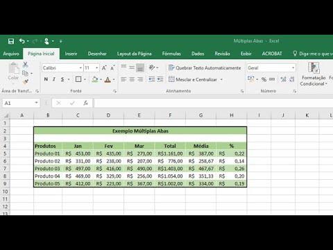
COMO FAZER UMA PLANILHA NO EXCEL (FÁCIL)
Microsoft Word 2010 - Basic User Guide - Lesson One - An Introduction
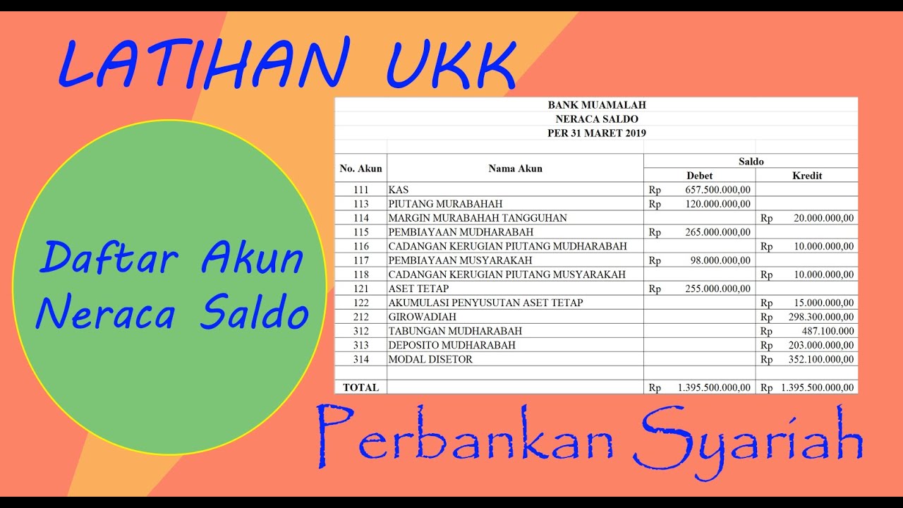
SIKLUS AKUNTANSI PERBANKAN SYARIAH: MEMBUAT NERACA SALDO AWAL MENGGUNAKAN APLIKASI MS EXCEL
5.0 / 5 (0 votes)
