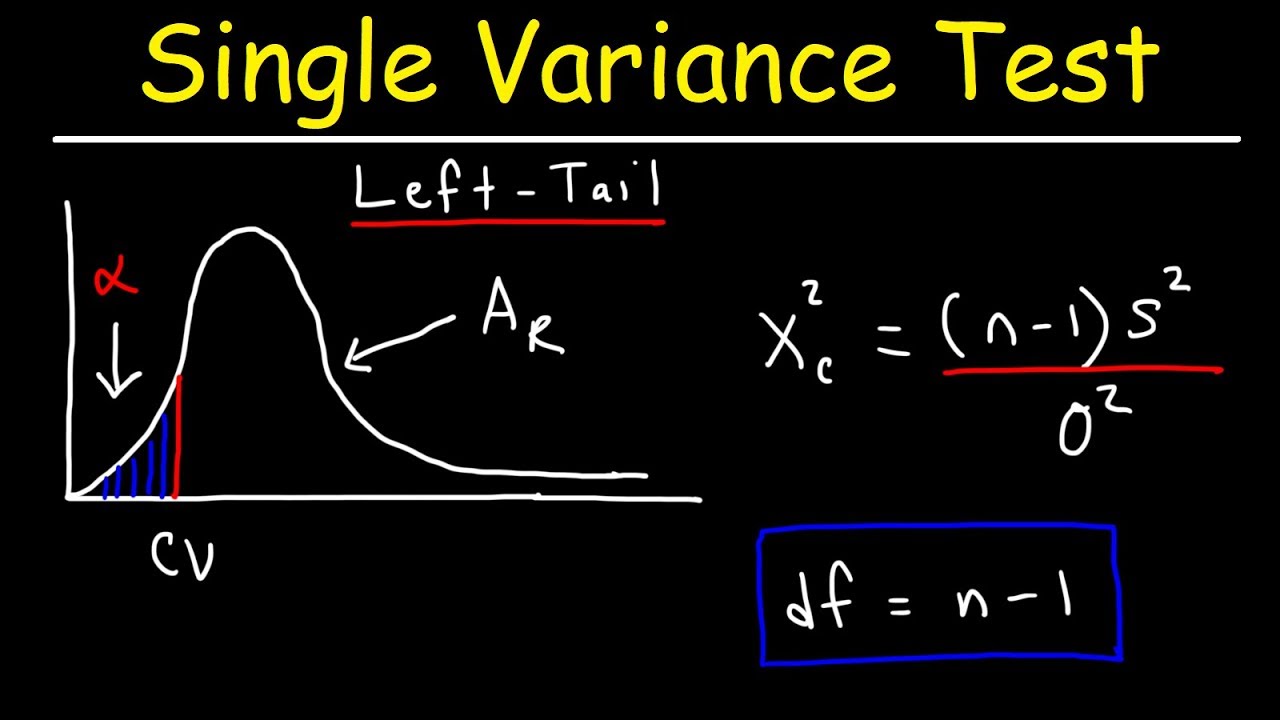
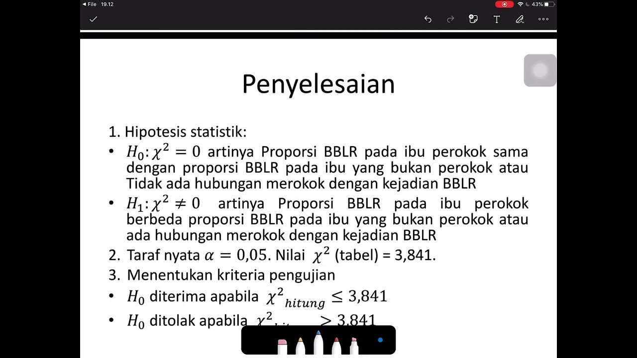
Statistics 101: Introduction to the Chi-square Test

Summary

In this video, we explore the basics of the Chi-Square test, a crucial tool in hypothesis testing. Designed for beginners in statistics, the video explains key concepts like random variation, expected versus observed frequencies, and interpreting results. The instructor uses real-world data and visual aids such as graphs to clarify these concepts. A simple example involving a fair versus loaded die illustrates the Chi-Square test step-by-step. The video emphasizes understanding data visually and sets the stage for a more complex problem to be solved in the next session.

Takeaways

• 📚 The video series is designed to introduce basic statistics concepts, particularly for those new to the subject or in need of a review.
• 🗣️ The presenter emphasizes the correct pronunciation of 'Chi-square' as 'Kai Square', like 'kite', to avoid common mispronunciations.
• 📈 The video discusses the use of various graphs such as line graphs, stacked bar charts, stacked percentage bar charts, stacked area charts, stacked percentage area charts, and spider diagrams to visualize and understand data better.
• 🔍 The Kai Square test is introduced as a method to determine if observed data varies significantly from expected data, which can indicate more than just random chance at play.
• 🎯 The presenter sets up a hypothetical scenario involving a fair and a loaded die to illustrate how the Kai Square test works in practice.
• ⚖️ The concept of 'null hypothesis' (H0) and 'alternative hypothesis' (H1) is explained, where H0 assumes no significant difference (e.g., the die is fair), and H1 assumes there is a significant difference.
• 📉 The video explains the process of calculating the Kai Square statistic through observed versus expected frequencies, squaring the differences, and dividing by expected values.
• 📊 The importance of the critical Kai Square value is highlighted, which serves as a threshold to determine whether to reject the null hypothesis based on the calculated Kai Square statistic.
• 🔢 The degrees of freedom, a key component in the Kai Square test, are discussed, and in the context of the die example, it is simply one less than the number of categories (5 in this case).
• 💯 The impact of the chosen P-value on the strictness of the test is demonstrated, showing how a more stringent P-value (e.g., 0.01 vs. 0.05) increases the critical Kai Square value needed to reject the null hypothesis.
• 🔑 The video concludes with a reminder that the next installment will apply the concepts learned to a more complex data set involving student enrollment data over five years.

Q & A

What is the purpose of the video series on basic statistics?

The purpose of the video series is to introduce and explain basic statistical concepts, particularly aimed at individuals who are new to statistics or need to review foundational ideas.

Why does the speaker prefer using the word 'stats'?

The speaker prefers using 'stats' because it has fewer 'S's and 'T's, reducing the likelihood of tripping over their own tongue while speaking, which they admit happens often.

What is the primary focus of the video on the chi-square test?

The video focuses on introducing the chi-square test, explaining its common misunderstandings, and demonstrating how to perform a simple chi-square test step by step.

What type of data is the speaker analyzing in the video?

The speaker is analyzing data on the number of undergraduate students at different class levels (freshman, sophomore, junior, senior, and unclassified) over a 5-year period at a regional university.

What is the main question the speaker is trying to answer with the data?

The main question is whether the variation in student headcount over the 5-year period is beyond what would be expected due to chance alone.

What types of graphs are discussed in the video to visualize data?

The types of graphs discussed include simple line graphs, stacked bar charts, stacked percentage bar charts, stacked area charts, stacked percentage area charts, and spider or radar diagrams.

What does the speaker notice about the junior and senior class levels in the data?

The speaker notices that the headcount for junior and senior class levels, as well as the unclassified students, has increased significantly over the 5-year period.

What is the correct pronunciation of 'chi-square' according to the speaker?

The correct pronunciation is 'Kai Square', rhyming with 'kite', not 'cheetah' or 'chai'.

What are the two categorical variables in the dice experiment presented in the video?

The two categorical variables in the dice experiment are the fairness of the die (fair or loaded) and the outcome of the dice rolls (numbers 1 through 6).

How does the speaker describe the relationship between the chi-square test and the observed versus expected data?

The speaker describes the chi-square test as a tool to help understand the relationship between two categorical variables by comparing the observed data (actual outcomes) with what is expected (theoretical outcomes), and determining if the variation is due to random chance or something else.

What is the significance of the P value in the context of the chi-square test?

The P value determines the level of tolerance for variation in the data. A lower P value means less tolerance for variation and a higher threshold for rejecting the null hypothesis, indicating that the observed data is significantly different from what would be expected by chance.

How does the speaker explain the concept of 'degrees of freedom' in the chi-square test?

In the context of the dice experiment, the degrees of freedom are explained as the number of categories minus one, which in this case is 6 (the six sides of the die) minus 1, equaling 5.

What is the null hypothesis in the dice experiment?

The null hypothesis in the dice experiment is that the die is fair, meaning that each roll has an equal chance of resulting in any of the six numbers.

What does the speaker conclude about the die based on the chi-square test results?

Based on the chi-square test results, the speaker concludes that the die is not fair, as the observed frequencies of the numbers differ significantly from what would be expected on a theoretically fair die.

What is the effect of changing the P value on the chi-square critical value?

Changing the P value affects the chi-square critical value. A lower P value results in a higher critical value, making it more difficult to reject the null hypothesis because the threshold for considering the variation as not due to chance is higher.

Outlines

00:00

📚 Introduction to Basic Statistics and Chi-Square Test

The speaker introduces a video series on basic statistics, clarifying that 'stats' will be used for ease of pronunciation. The videos are aimed at beginners or those needing a review. The first topic is the Chi-Square test, often misunderstood, and the speaker plans to set up a complex problem to be solved in a subsequent video. The Chi-Square test will be introduced with a simple example before tackling the complex problem. The context involves analyzing changes in undergraduate student headcount at a university over five years, with the goal of determining if observed variations are due to chance. The speaker emphasizes the natural random variation in such data and sets the stage for using graphs and the Chi-Square test to analyze it.

05:02

📊 Exploring Data Visualization Techniques

This paragraph delves into various data visualization methods to better understand the student headcount data. The speaker extols the virtues of graphs for their ability to enhance data comprehension. The options discussed include simple line graphs, stacked bar charts, stacked percentage bar charts, stacked area charts, stacked percentage area charts, and spider or radar diagrams. Each visualization technique offers a unique perspective on the data, from tracking changes over time to comparing proportional enrollments and relative percentages. The speaker provides examples of how these methods can reveal insights into the data, such as the increasing headcount of juniors, seniors, and unclassified students compared to freshmen and sophomores.

10:03

🎲 Understanding the Chi-Square Test with a Dice Experiment

The speaker introduces the Chi-Square test with a dice experiment to illustrate the concept in a relatable way. The test is used to examine the relationship between two categorical variables, such as the outcome of dice rolls. The experiment involves rolling a die 100 times a day for six days, recording the frequency of each number. The expected outcome is that each number would appear 100 times if the die is fair. The Chi-Square test will compare the observed frequencies with the expected frequencies to determine if the variation is due to random chance or if it suggests the die is loaded. The explanation includes setting up a null hypothesis (the die is fair) and an alternative hypothesis (the die is not fair), and it touches on the concepts of P values and degrees of freedom, although it does not delve into their technical definitions.

15:05

🔢 Calculating the Chi-Square Statistic

The speaker provides a step-by-step guide to calculating the Chi-Square statistic using the observed and expected frequencies from the dice experiment. The process involves subtracting the expected frequency from the observed frequency, squaring the result, and then dividing by the expected frequency. The outcomes of these calculations are then summed to obtain the Chi-Square value. The speaker emphasizes the simplicity of the math involved and explains that the final Chi-Square value will be used to make a statistical conclusion about the fairness of the die.

20:06

🎯 Interpreting the Chi-Square Test Results

The paragraph explains how to interpret the Chi-Square test results by comparing the calculated Chi-Square value with a critical value obtained from the Chi-Square distribution. If the calculated value exceeds the critical value, the null hypothesis is rejected, suggesting the die is not fair. The speaker uses an example with a Chi-Square value of 12.26 and a critical value of 11.07, leading to the rejection of the null hypothesis. The explanation includes the impact of the P value on the strictness of the test, with a lower P value requiring greater observed variation to reject the null hypothesis. The speaker also demonstrates how changing the P value from 0.05 to 0.01 increases the critical value, thus affecting the conclusion of the test.

25:07

📘 Recap and Preview of Upcoming Video Content

In conclusion, the speaker summarizes the Chi-Square test, emphasizing its purpose for analyzing the relationship between two categorical variables and comparing observed data with expected outcomes to determine if variations are due to random chance. The speaker also previews the next video, which will apply the Chi-Square test to the university enrollment data introduced earlier. The goal of the next video will be to assess whether the variations in student headcount can be attributed to random chance or if there are other factors at play.

Keywords

💡Statistics

Statistics refers to the branch of mathematics that deals with the collection, analysis, interpretation, presentation, and organization of data. In the context of the video, statistics is the overarching theme, as the script discusses various statistical concepts and methods, such as hypothesis testing and the chi-square test, to analyze and interpret data, particularly in the field of institutional research.

💡Chi-Square Test

The chi-square test is a statistical test used to determine if there is a significant difference between the expected frequencies and the observed frequencies in a dataset. The video provides an in-depth introduction to this test, explaining its purpose, how it is conducted, and how to interpret its results. The test is used to analyze the relationship between two categorical variables, as demonstrated in the script with an example involving dice rolls.

💡Hypothesis Testing

Hypothesis testing is a statistical method used to make decisions about populations based on sample data. The video script introduces the concept of hypothesis testing by explaining the null hypothesis (H0) and the alternative hypothesis (H1). It uses the example of a fair versus a loaded die to illustrate how to set up and test hypotheses, and how to interpret the results to determine if the observed data is significantly different from what would be expected by chance.

💡Observed Frequency

Observed frequency refers to the actual data collected during an experiment or study. In the video, observed frequency is used in the context of the chi-square test, where the script describes how to calculate the difference between the observed frequencies of dice rolls and the expected frequencies to determine if the die is fair or loaded.

💡Expected Frequency

Expected frequency is the frequency of an event that would be expected if the null hypothesis were true. The script explains how to calculate expected frequencies for each category in a dataset, using the assumption that a die is fair, and each number should appear 100 times out of 600 rolls as an example.

💡Degrees of Freedom

Degrees of freedom (DF) is a statistical concept that represents the number of values that can vary freely in a set of data. In the video, the degrees of freedom are used in the context of the chi-square test, where the script explains that for a simple chi-square test with six categories, the degrees of freedom would be 5 (6 - 1).

💡Critical Value

A critical value is a value of a test statistic that determines the threshold for rejecting the null hypothesis in a statistical test. The video script discusses how to find the chi-square critical value using Excel and explains that if the calculated chi-square value exceeds this critical value, the null hypothesis is rejected.

💡P-Value

The p-value is the probability that the observed results (or something more extreme) would occur if the null hypothesis were true. The script explains the concept of p-values in the context of setting a level of confidence for the statistical test, and how changing the p-value affects the critical value and the decision to reject or accept the null hypothesis.

💡Graphs and Data Visualization

Graphs and data visualization are methods used to represent data in a graphical format to make it easier to understand and interpret. The video script discusses various types of graphs, such as line graphs, bar charts, and spider diagrams, and how they can be used to visualize changes in student headcount over time, helping to understand patterns and variations in the data.

💡Categorical Variables

Categorical variables are variables that can take on one of a limited, and usually fixed, number of possible values, assigning each individual or case to a particular group or category. The script emphasizes that the chi-square test is used to analyze the relationship between two categorical variables, such as class levels (freshman, sophomore, etc.) and years in the context of student enrollment data.

Highlights

Introduction to the Chi-Square test, a fundamental statistical method for hypothesis testing.

Explanation of the pronunciation and spelling of 'Chi-Square' to avoid common mistakes.

Overview of the Chi-Square test's purpose in understanding the relationship between two categorical variables.

Description of the test's application in comparing observed data with expected outcomes.

Introduction of a hypothetical scenario involving student enrollment data at a university to illustrate the test.

Discussion on the natural random variation in data and how Chi-Square helps determine if observed variation is beyond chance.

Presentation of various graphing options like line graphs and bar charts to visualize data effectively.

Analysis of student headcount data over five years using different graphical representations.

Explanation of how to calculate the Chi-Square statistic step by step using a dice-rolling experiment.

Clarification of statistical terms such as 'null hypothesis' and 'alternative hypothesis' in the context of the test.

Importance of the P-value in determining the level of confidence in the test results.

Calculation of the Chi-Square critical value using Excel for making statistical inferences.

Interpretation of the Chi-Square test result comparing the test statistic to the critical value.

Impact of changing the P-value on the stringency of the test and its critical value threshold.

APA format guidelines for reporting Chi-Square test results in academic writing.

Summary of the Chi-Square test process from hypothesis formulation to conclusion drawing.

Preview of the next video's content, which will involve a more complex application of the Chi-Square test to enrollment data.

Transcripts

[Music]

hello and welcome to my video series on

basic statistics now two notes before we

get going number one I will most often

just use the word stats there are fewer

S's and T's crammed together in stats

and therefore I am less likely to trip

over my own tongue which happens often

number two these video are geared

towards individuals who are relatively

new or just need to review the basic

concepts in stats so if you have

advanced study in quantitative methods

these videos are probably a bit below

what you would need also if you do have

advanced study in quantitative methods

just keep in mind that I am simplifying

some of the concepts for those who are

new to the topic so all that being said

let's go ahead and Dive Right

In

in this video we will be doing an

introduction to the kai Square test this

is one of the most often

misunderstood tests in hypothesis

testing so we're going to do a couple

things we're going to set up a more

complex problem that we will actually

solve in the next video but we'll talk

about it in this video after we talk

about that data we'll look at some

graphs that help us understand that data

better and then we will actually do a

simple Ki Square test

step by step so you can see exactly how

the numbers are calculated which are

actually fairly simple and then how we

interpret that so let's go ahead and

talk about our

problem now again this problem will be

solved in the next video in this video I

will actually be doing a simple example

that we will then apply to this more

complex problem so we'll see this more

again in part

two so you work in the office of

institutional research at a small but

growing Regional 4year University over

the past 5 years the number of

undergraduate students at each level so

freshman sophomore Junior and senior and

then we have unclassified students which

are sometimes high school students or

others um has changed so we have had

variation in our student headcount over

this 5year

period now here are our questions now

even though some headcount random

variation is

inevitable is that variation beyond what

we would expect due to chance alone now

there is a lot packed into that question

and I want to explain a couple of things

just out in the world when we count the

occurrences of things if we count An

Occurrence maybe today and then we count

the same thing tomorrow and then we

count the same thing the day after that

and the day after that there's going to

be a natural random variation in the

number that we count so maybe I go out

to a busy stoplight and I count the

number of cars that go through it during

a 15minute interval say during rush hour

well if I do the same thing tomorrow I'm

going to get a different number if I do

the same thing the day after that I'm

probably going to get a different number

but those numbers are probably going to

be close together even though they vary

a little bit just you know randomly so

what we're trying to ask here is is that

variation

beyond what we would expect just due to

the normal random chance

variation now what types of graphs can

we use to better visualize our

data and how can a Ki Square test help

us rule out that variation due to chance

alone so where is the threshold by which

we can say wait a minute that change is

just beyond what we'd expect due to

chance

alone so here is our student headcount

now this is actual data by the way I did

not make this up so we have the years

2007 through

2011 then we have the class levels

freshman sophomore junior senior and

then we have the unclassified and this

track the student headcount or

enrollment you can think of it during

the fall semester of each one of these

years so go ahead and take a look at

that and we'll talk about what we

see but one thing I noticed is that for

Junior and senior the headcount goes up

quite a bit over that amount of time and

the same thing for in classified if I

look at freshman and sophomore it kind

of goes up and down there is no real you

know pattern as far as straight up or

straight

down now let's go ahead and do some

graphing options so we can visualize

this data

better now one of my credos is graphs

are your friend graphs are awesome use

more

graphs take advantage of our ability to

understand data visually a column of

numbers is one thing but making it

visual is a whole another thing and that

can really help with your classmates or

your instructor or your co-workers or

your Dean or whoever else you might be

presenting this to take advantage of our

ability to understand data visually so

in this problem we're going to consider

simple line

graph a stacked bar

chart a stacked percentage bar chart a

stacked area

chart a stacked percentage area chart

and then a spider or radar diagram and

we're going to talk about what each one

does for us as far as interpreting or

understanding our data

better so here's our simple line graph

and we have our five class levels over

on the right hand side denoted by each

line now as you can see if you start at

the bottom the special uh category seems

to go up over time the junior which is

the green line goes up the senior line

which is the purple goes up over time

but then we have sophomore which kind of

goes up and down and then the same thing

for the Freshman it starts up goes down

and comes up again and then kind of goes

down again so when we talk about

variation in our data across the years

this is what we're talking about now

because of the Natural Way enrollments

work and other things in you know in

society and nature work there's going to

be some natural random variation we

cannot expect expect unless we do some

serious quota filling to have the exact

same enrollment every year so we're

going to have natural variation now what

we're trying to figure out is is that

variation within what we we would expect

by just sort of random chance

alone now here is a stacked bar chart

which is another way of looking at our

data So within each year we have the

number of students in each class level

and then they're stacked on top of each

other so what does this do for us you

know that's new well it helps us see

proportional enrollment so you can see

that the Freshman which is there in the

blue bar not only can we see its pattern

over time you know down a little bit up

and then down a little bit but we can

also see its size relative to the other

class levels so it seems to be about

twice as much as the sophomore which is

about twice as much as the the junior

depending on the year you're looking at

and then Senior and our special category

so it helps us see relative in this case

enrollments you know as one class level

is compared to

another now here is our stacked

percentage chart now of course in this

case each class level is described by

the percentage of the total enrollment

it occupies for any given year so if we

look in 2007 we can see that freshmen

were approximately

38% of our total undergraduate

enrollment or headcount in 2008 that

went down to about maybe

33% by the time we got to 2011 we're

almost all the way down to

30% now of course the entire enrollment

takes up 100% so it's all relative here

again and you can see that the special

color there at the very top gets bigger

so it takes up a larger percent of our

enrollment same thing for seniors it

appears and

juniors and then sophomores seem to

narrow in their percentage as we go

across time so this helps us look at

relative percent for each

year now here is a stacked area chart

now this is very similar to the Stacked

bar chart except we take that data and

we go all the way across the graph with

it so this tells us a few things if we

look at the very top of the graph we can

see that it increases so what we can say

is that our overall head count our

overall student enrollment increased

over this time period from you know in

the mid

1400s up to above

1,600 now as far as the individual bands

of course those represent each each

class level so if we look the senior the

purple seems to widen over time the

junior the green seems to widen over

time the sophomore level seems to narrow

a bit and the Freshman seems to narrow a

bit so again with this visual

information we can sort of make you know

some ideas in our head about how this

has changed over time it seems that our

freshman and sophomore enrollments went

down a bit but our Junior and senior in

special category enrollments went up

over this time and actually with this

University there's a I have a hypothesis

at least why that happened but maybe

we'll talk about that in the next

video now here is our stacked percentage

area chart and this is very similar to

our stacked percentage bar chart where

each band represents a percentage of the

total so again you can see that overall

The Freshman seems to narrow as a

percentage same thing with the

sophomore percentage and the junior you

got to look at two things here does it

get wider and sort of its direction so

it does seem to get whiter and then same

thing with the senior there in the

purple and the special category there on

top so what can can we say about this

well it seems that our freshman and

sophomores

combined are taking up a smaller

percentage of our overall undergraduate

enrollment and then our junior senior

and special categories are taking up a

larger percent over this time so again

we have variation in our enrollment but

our question is is it within just random

chance variation or is there something

else going

on now the last one we're going to look

at is the spider diagram and again this

is an often underused diagram that I

think can be very helpful now of course

each grade level is represented by a

different color and in the center we can

call that a hub kind of like the Hub of

a wheel if You' like and then radiating

out are the years so each spoke coming

out of that Center is a year so 2007 08

09 2010 and

2011 then of course we plot the number

of students in each grade level along

that spoke now what does this tell us

new well if you notice as we swing

around the spider diagram as we get

towards 2010 and

2011 we have like a bulge in the special

the Juniors and the seniors so the the

lighter blue the green and the purple

and if you remember other graphs that

was apparent in our areas in stacked

bars because the Juniors the seniors and

the special cat ategory we becoming a

greater part of her overall

enrollment then if you look at the red

it doesn't change a whole

lot over time sometimes it comes in a

bit and goes back out and comes in a bit

and goes back out but not by a whole lot

and then the blue starts way out almost

all the way to 600 students comes back

in to 500 in 2008 goes back out to the

middle stays in the middle and then

comes back in again at 2011

so it helps us sort of see bulges in our

sper our spider or radar diagram to see

where our changes have

been okay so let's actually get to the

heart of this video and that is what is

a Kai Square

test now first and

foremost make sure you pronounce it

[Music]

correctly it is Kai Square as in kite

not ch as in cheetah not a chi

square or

chai as in chai T it's not chai square

it is Kai Square so I've been in about

10 different stats classes between

undergraduate and all my graduate work

every class every one of them someone

has said I don't understand the chi

square or I have a question about the

chai square it's Kai Kai Square as in

kite so don't be that person in your

class okay now what does it do it helps

us understand the relationship between

two

categorical variables and that's very

important they have to be categorical

variables so what do I mean by that well

grade level that's one example in this

case so we have freshman sophomore

junior senior and then special or

unclassified um sex male or female if we

think of it as a binary

category um age group so we could have

you know you've probably seen them are

you in the age group 18 to 25 or 26 to

35 or 36 to 45 whatever so those are

categories if they're put in

groups years of course we have years in

this example Etc so the important thing

here is it has to be categorical

variables now Kai squares involve the

frequency of events or the count so

we're only dealing with counting things

we are counting members of these

categories we're not dealing in percents

we're not dealing in anything like that

we are dealing in frequencies

counting now it helps us compare what we

actually

observed with what we

expected okay observed versus

expected often times using population

data and I don't want to go into all

that right now but you know that's every

member of a certain category we denote

so that's a population or theoretical

data and actually when we do our example

we're going to be using a theoretical

data event I guess you could

say now Kai squares assist us in

determining the role of random chance

variation between these categorical

variables so the relationship is going

to change but the question is is that

change within a certain limit we set

that would account for just random

variation and finally we use the Ki

Square distribution now if that just

went whatever your head do not worry for

this video it's not important just know

that we use use it and I put it in here

just to be technically correct and

within that we use what's called a

critical value which I'll explain here

in a little bit to accept or

reject our

hypothesis okay so if I'll just talk

about hypothesis and kisore

distributions or critical values or have

your mind going in Crazy directions

right now don't worry in the example

we're going to do is going to be so

Crystal Clear step by step that uh

you'll have it down pat

now just look at our head count changes

over time again so we can see we have a

couple of categories that go seem to go

up over time almost in like a very flat

straight line and then we have a couple

sophomore and freshmen that kind of

Bounce all over the place so we have

variation and we just want to know are

these categories grade level and year

the variation that occurs is it due to

random chance alone or is there

something else going on in this

data now in this video we're going to

use a very simple experiment it's very

common when talking about the Ki square

and that is the dice experiment and I'm

going to set it up maybe a little bit

differently than other people have so

here is our

example let's say I have two Dy in my

hand okay and just in case you maybe are

not familiar you know D or the six-sided

squares that are often used in games

especially like gambling games and they

have you know one through six on each

side so let's say I have two Dy in my

hand one is fair and the other is 156

loaded that means it favors the numbers

five and six due to alterations in its

weight so some people that cheat at

casinos swap out the

actual uh casino dice or dice with

weighted dice to get the numbers they

want okay so I give you two of them and

one is fair and one is

loaded now I ask you to determine if

it's the fair die or the loaded die I

just gave you and I want you to be

95% confident in your

conclusion now to do that what you're

going to do is I'm going to ask you to

do is over the next 6 days I want you to

roll that dot okay 100 times each

day for a total of 600 rows okay and

then record how many times each number

occurs over those 600 rolls so you're

going to 100 rolls each day for 600 for

6 days 600 total rolls keeping count a

frequency of how many times each number

comes

up now let's assume

okay that the die I gave you is fair

let's assume that what would we expect

to happen What Would We theoretically

expect to happen over these 600

rows now if the die is fair if we roll

it 600 times and we have six numbers on

the die we would theoretically expect

each number to come up 100 times so so

six numbers 600 rolls each one has the

same probability of coming up so

theoretically we would expect 100 of

each number to

occur so how we going to State this

hypothesis and again this is one of the

more complicated slides to just hang

with

me first we have What's called the null

hypothesis and that's represented by H

subz so if you've been in St St class

you've probably seen something like this

now our null hypothesis is that the die

is

fair then we have our our alternative

hypothesis which is denoted by H sub

one and our alternative hypothesis is

that the die is not

fair okay so we have the null that says

the die is fair we have the alternative

that says the D is not fair pretty

straightforward

now what is the everyday sort of English

way of saying

this now is the variation in our

observed data simply due to

chance or is the variation beyond what

random chance should

allow or how far can our data vary

before we have to reject the null

hypothesis ois and conclude that the die

is not fair which is our our

alternative so we're going to have some

variation but we need to know if that

variation occurs within limits we

set now I asked you to be 95% confident

so that creates what's called A P value

of

0.5 so again if that P value concept

kind of goes over your head don't worry

about it too much now another way of

thinking about the P value is what level

of Tolerance are we willing to put on

this

variation if our tolerance is pretty

loose we might have a P value of 0.1 or

sort of

10% if we want the tolerance for the

variation in our data to be very narrow

we want to be very strict

we might choose a P value of

0.1 or

1% so I've sort of pick the medium which

is 05 which is often you the most

commonly common use commonly used in a

lot of social science

research okay so degrees of freedom oh

goodness this is one of those Concepts

that gets flown around flung around in

stats classes and never gets explained

at least in my experience very well and

guess what I'm not going to explain it

in this video either now for this kind

of for this test our degrees of Fe

Freedom DF are simply the number of

categories we have which is six we have

six numbers minus one okay so in this

example just kind of take it as it is

that our degrees of freedom are 6 - 1

which equals 5 now in the next video

when we have more complex categories the

degrees of freedom will be figured a bit

differently but for this example it's

just 6 - 1 or five now we have a concept

called the kai Square critical value

well what is that well the kai Square

critical value is sort of um the

threshold it is the point where we just

have to conclude that our variation is

too great to be explained by chance

alone and therefore we'd have to reject

our n hypothesis over there so the

easiest way to find this actually is in

Excel Excel has a built-in function sort

of the kai inverse or CH hii I in v and

then you just give it two inputs you

give it your P value which in our case

is

0.005 then you give it your degrees of

freedom which in our case is five then

it spits back a value a critical value

of

11.07 so when we do this kind of keep

that number in the back of your mind our

threshold for our Ki Square critical

value is going to be

117 so what that means is that if our D

Kai square is greater than

11.07 then we have to reject our null

hypothesis and claim that the die is not

fair the variation is just beyond what

we would expect by normal random chance

or normal random variation so if we get

a Kai Square that's greater than

11.07 we got to throw the null

hypothesis in the garbage and just

accept the alternative hypothesis which

states the die is not fair so let's go

ahead and do this step by

step okay so here is our expected

frequency which we talked about now on

the right hand hand side is what our

data actually produced these are our

actual observations so 6 days later you

come to me and say here are my

observations so the number one came up

111 times the number two came up 90 3 81

Etc and of course that adds up to 600

total rolls so those are our observed

frequencies when we actually did the

experiment so here's the first step in

figuring out our Kai Square the math is

very very easy okay so I know you're

smart and you can do it so let's go

ahead and just do it step by step the

first step is we take our observed our

observation minus what we expected so as

you can see on the right hand side it's

simple subtraction we take our observed

which in the first case is 111 minus our

expected which was 100 because we

expected to be a fair die so 111 minus

100 is 11 and then we just do that all

the way down that column that's it

that's step one observed minus

expected in the next step we take that

observed minus the expected and square

it that's it so for number one remember

we had 111 - 100 which was 11 and then

in this step we just Square it which is

121 then we do that for each of our

numbers so step one we subtract step two

we Square it that's

it now in step three we take what we got

in step two which was the

squaring and we divide that by what we

expected which is e okay so in all of

our cases we expected 100 this is not

this is actually very simple division

it's just moving the decimal place so

for the number one we had 121 minus 100

that's

1.21 for number two it's just well one

and for number three we had

3.61 and for number four we had

0.04 and on down five and six so that's

step three just remember Step One is

subtraction step two we square that and

the step three we divide that by our

expected which in this case was 100 so

it's very

easy now in step four we just add all

those up so in our right-and column

again we had 1.21 1 3.61 04 Etc we just

add all those up that's what the

summation sign at the top of the slide

means and guess what folks we just did

our Kai Square we're

done at least at least with the math

part so our Ki Square value for this

experiment was

12.26 of course that doesn't mean

anything yet until we actually interpret

it but the kai Square value for this is

12.26 now remember our critical Ki

Square value was

11.07 now guess what 12.26 is greater

than

11.07 so therefore our die critical

value is greater than

11.07 so we have to reject our null

hypothesis which said the die is fair

and claim that the die is in fact not

fair so we have to accept our

alternative hypothesis because our Kai

Square was greater than our critical Ki

square based on our Excel

formula so how do we interpret that

result now if we actually use the APA

format which I encourage you to do

depending on your discipline of course

what we would say is that the observed

frequency of each number on the die

differed significantly from what would

be expected on a theoretically Fair

die of course we have our Kai Square

Five is our degrees of freedom n is the

number of times we rolled the die and

that equal

12.26 and our P value was

05 so if you were writing this in a

journal that's exactly how it would look

in apa

format now our problem Ki Square was

12.26 our critical Ki Square was 11.07

which is therefore our variation was too

great to be explained by chance alone

therefore we must reject uh our null

hypothesis which is the diph and accept

H1 which was our alternative hypothesis

and say the die is not fair so we are

95% confident that you have the loaded

die in your

hand now I want to talk about just the

effect of choosing a P value remember I

said the P value was sort of how strict

we're willing to be on accepting random

variation if we change the P value we're

going to sort of change the threshold of

what we're willing to accept as random

chance now this is the same slide I just

changed a few numbers so null hypothesis

is still the die is fair alternative is

the die is not

fair same interpretation okay we're

talking about variation

here here's what we changed instead of

being 95% confident I want you to be

99% confident so we're going to have a P

value not 05 but now it's going to be

0.01 so we're going to be much much more

strict on interpreting our variation now

what that means is that we're going to

need a lot more variation in our

observations in order to reject our null

hypothesis we're going to need much more

variation in our observations to reject

our null hypothesis because we've

selected a much more strict P value now

degrees of freedom are the same now for

the kai Square we changed our P value so

we're going to have a new critical value

so when we put this into Excel we

changed that to 0.01 degrees of freedom

are five now our critical value is

15.09% to go over that threshold because

we've picked such a strict P

value so therefore if our die Kai square

is greater than

15.09% on a theoretically Fair die and

everything there is the same five

degrees of freedom 600 rolls our problem

Kai Square was 12.26 that didn't change

but our P value did so we have a p of

01 so our problem Kai Square was

12.26 our critical Kai square with a P

value of

01 was now

[Music]

15.09% that threshold therefore our

variation was not too great to be

explained by chance alone therefore in

this case we have to accept our null

hypothesis and conclude the die is fair

and we are 99% confident that you have

the fair

die now wait a

minute you have the same Dy in your

hand but in the first case when P was

05 we concluded you had the loaded

die now with a p of

01 we conclude you have the

farad what now this is my point on

changing the P value or changing the

strictness with which we are willing to

explain

variation so with a p of

05 we did not need as much variation

to

overcome the critical value as you

notice the critical value went up

significantly when we changed the P to

0.01 so it's just much more strict we

have to have more variation to cross

that sort of 99% confidence because we

selected such a low P

value all right just a quick review what

is a Ki Square test remember it is Ki

Square not not CH Square or chai square

it's Kai and kite it helps us understand

the relationship between two categorical

variables that's

important Ki squares involve the

frequency of events the count so in this

case we were counting the number of

times each number comes up it helps us

compare what we actually observed with

what we

expected Kai squares assist us in

rejecting or ruling out to some extent

random chance variations between

categorical

variables and we use the kai Square

distribution which we didn't talk about

it's not important to what we're doing

um to accept or reject our hypothesis

regarding random chance now basically

what that means there is that we were

able to put into Excel our degrees of

freedom and our P value and it generated

a critical Kai Square value that we have

to surpass in order to reject our null

that's all that little thing means to on

there okay so that's

review now just reminder in our next

video we will actually be looking at the

data we started with so look in this

case instead of having a die with six

numbers on it we have five class level

categorizations so freshman through

unclassified then we have five years so

we have five grade levels and five years

for our categories and then we're going

to try to determine are we are going to

determine whether or not the variation

present in this

data can be explained just by you know

random chance just the random chance

that comes with

enrollment all right so that is our

in-depth introduction to the kai Square

hopefully you learned a lot and I look

forward to seeing you again in our next

video when we look at that enrollment

data in a more complex example again

thank you very much for watching I look

forward to seeing you again next

[Music]

time