Week 4-Lecture 23
Summary
TLDRThis lecture explores the optimal map detector for AWGN channels, focusing on decision regions in signal space that minimize error probability. It explains how detectors partition the space and use correlation and match filters for implementation. The discussion includes the impact of equiprobable and non-equiprobable messages on decision regions, with examples illustrating the geometrical representation of signals in vector space. The lecture concludes with calculating the probability of error for both equiprobable and non-equiprobable cases, highlighting the challenges of high-dimensional signal spaces.
Takeaways
- 📡 The optimum map detector for AWGN channels is derived and its implementation is based on correlation and match filters.
- 🔍 To determine the error probability of the optimum receiver, decision regions in the signal space must be established.
- 📏 The N-dimensional signal space is partitioned into M regions, each corresponding to a message signal, aiming to minimize the error probability.
- 📶 The decision region R_k includes all points in the N-dimensional space where the probability of message m_k given observed vector x is greater than for any other message.
- 📉 For equiprobable messages, the decision regions are determined by the perpendicular bisectors of the lines joining signal points, reflecting the spherical symmetry of Gaussian noise.
- 📊 The decision function for an AWGN channel can be expressed as the argument minimum of a norm of the difference between the received vector and signal vectors.
- 📈 Non-equiprobable messages lead to weighted decision regions, favoring messages with higher probabilities, which is reflected in the decision function by the log of the message probabilities.
- 📐 In higher-dimensional signal spaces, visualizing decision regions becomes difficult, and the calculation of error probabilities is more complex.
- 🔢 The probability of correct detection is calculated based on the region where the received vector falls, which is easier with defined decision regions.
- 📉 The probability of error is found by subtracting the probability of correct detection from 1, and can be simplified for specific cases such as equiprobable messages.
Q & A
What is the purpose of decision regions in signal space?
-Decision regions in signal space are used to partition the N-dimensional signal space into M regions, where M is the number of message signals. This partitioning is done to minimize the probability of error by assigning received signals to the most likely transmitted message based on their proximity in signal space.
How does the optimum receiver determine the decision regions?
-The optimum receiver determines the decision regions by choosing them to minimize the probability of error. For a MAP (Maximum A Posteriori) detector, the decision region R_k includes all points in the N-dimensional space for which the probability of message m_k given the observed vector x is greater than the probability of any other message m_j given x, for all j not equal to k.
What is the significance of equiprobable messages in decision region formation?
-When messages are equiprobable, the decision regions are formed by the perpendicular bisectors of the lines joining the signal points. This is because the decision is made in favor of the signal that is closest to the received vector x, and for Gaussian noise, which has spherical symmetry, the boundary between decision regions will be equidistant from the signal points.
How does the presence of non-equiprobable messages affect decision regions?
-In the case of non-equiprobable messages, the decision regions are biased in favor of the message with a higher probability. This is reflected in the decision function by the inclusion of the log of the probability of the message, which results in weighted decision regions that favor the more probable messages.
What is the role of the Q function in calculating the probability of correct decision?
-The Q function plays a crucial role in calculating the probability of correct decision in the presence of Gaussian noise. It is used to determine the probability that the noise component will not cause the received vector x to fall into the wrong decision region, thus ensuring a correct decision is made.
How is the probability of error calculated given the decision regions?
-The probability of error is calculated by considering the complement of the probability of correct detection. The probability of correct detection is the probability that the received vector x belongs to the correct decision region R_j, given that message m_j was transmitted. The unconditional probability of correct detection is the sum of these conditional probabilities, and the probability of error is 1 minus this sum.
What is the significance of the perpendicular bisector in the context of decision regions?
-The perpendicular bisector of the line joining two signal points is significant because it forms the boundary between two decision regions. This boundary is the set of points equidistant from the two signal vectors, which is a straight line perpendicular to the line joining the signal points and passing through the midpoint at a distance determined by the probabilities of the messages.
How does the dimensionality of the signal space affect the visualization and calculation of decision regions?
-As the dimensionality of the signal space increases, the visualization of decision regions becomes more complex and potentially impossible beyond two dimensions. Similarly, the calculation of the probability of error becomes more challenging and may require more advanced mathematical techniques or computational methods.
What is the impact of the noise power spectral density on the decision regions and the probability of error?
-The noise power spectral density affects the decision regions and the probability of error by influencing the distribution of the noise in the signal space. Higher noise power spectral density leads to a larger spread of the noise, which can cause the received signal to be more likely to fall into the wrong decision region, thus increasing the probability of error.
Can you provide an example of how decision regions are calculated for non-equiprobable messages?
-For non-equiprobable messages, the decision regions are calculated by considering the log of the probability of each message in the decision function. For example, if the probability of message m_2 is higher than m_1, the decision region R_2 will be biased towards S_2, making it larger. The boundary is determined by the condition where the squared distance from the received vector x to S_1 is equal to a constant c, which is derived from the probabilities of m_1 and m_2.
Outlines

هذا القسم متوفر فقط للمشتركين. يرجى الترقية للوصول إلى هذه الميزة.
قم بالترقية الآنMindmap

هذا القسم متوفر فقط للمشتركين. يرجى الترقية للوصول إلى هذه الميزة.
قم بالترقية الآنKeywords

هذا القسم متوفر فقط للمشتركين. يرجى الترقية للوصول إلى هذه الميزة.
قم بالترقية الآنHighlights

هذا القسم متوفر فقط للمشتركين. يرجى الترقية للوصول إلى هذه الميزة.
قم بالترقية الآنTranscripts

هذا القسم متوفر فقط للمشتركين. يرجى الترقية للوصول إلى هذه الميزة.
قم بالترقية الآنتصفح المزيد من مقاطع الفيديو ذات الصلة

Bayesian Learning
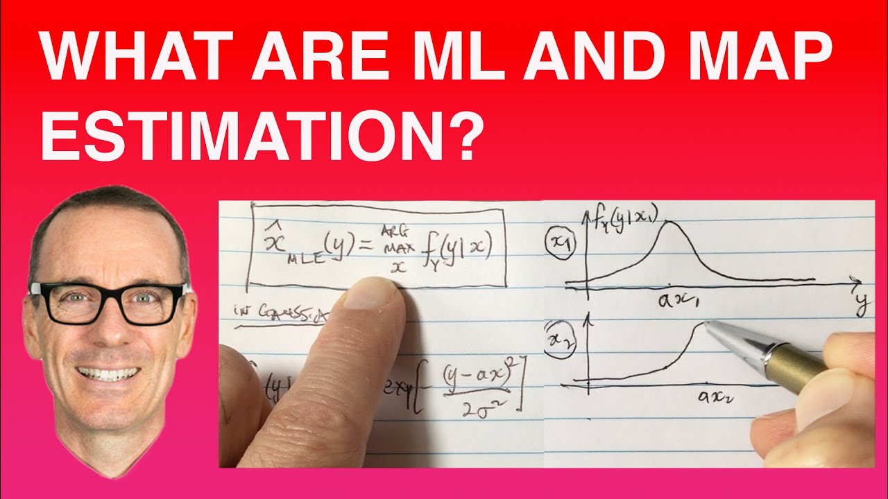
What are Maximum Likelihood (ML) and Maximum a posteriori (MAP)? ("Best explanation on YouTube")

Channel Models in Wireless Communication

Cell Sectoring and Cell Splitting | Improving Coverage and Capacity In Cellular System

RO11 Teori Permainan (Game Theory)
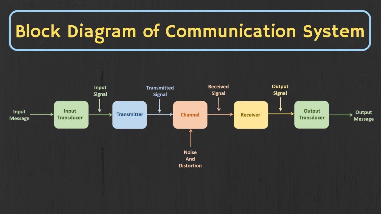
Introduction to Analog and Digital Communication | The Basic Block Diagram of Communication System
5.0 / 5 (0 votes)
