What are Maximum Likelihood (ML) and Maximum a posteriori (MAP)? ("Best explanation on YouTube")
Summary
TLDRThis script explores the concepts of Maximum Likelihood Estimation (MLE) and Maximum A Posteriori (MAP) in the context of signal processing. It uses the example of a system with a constant 'a' and additive white Gaussian noise (AWGN) to illustrate how to estimate an unknown variable 'x' from measurements 'y'. The video explains the process of finding the MLE by maximizing the probability density function (PDF) of 'y' given 'x', and contrasts it with MAP, which incorporates prior knowledge about the distribution of 'x'. The script clarifies the difference between the two by visualizing the PDF plots for various 'x' values and how they are affected by the measurement 'y-bar'. It concludes by noting that MLE and MAP are often the same in digital communications where symbols are equally likely.
Takeaways
- 📚 The script discusses two statistical estimation methods: Maximum Likelihood Estimation (MLE) and Maximum A Posteriori (MAP).
- 🔍 MLE is an estimation technique where the estimate of a parameter is the one that maximizes the likelihood function given the observed data.
- 📈 The script uses the example of a system with a constant 'a' and additive white Gaussian noise (AWGN) to explain MLE, where measurements 'y' are taken to estimate an unknown 'x'.
- 🌡️ Practical applications of the discussed concepts include estimating temperature in IoT devices, digital signal processing, and radar tracking.
- 📉 The likelihood function for a Gaussian noise model is given by a normal distribution with mean 'a times x' and variance 'sigma squared'.
- 📊 To find the MLE, one must plot the likelihood function for various values of 'x' and identify the peak that corresponds to the measured 'y'.
- ✂️ MAP estimation incorporates prior knowledge about the distribution of 'x', in addition to the likelihood function, to find the estimate that maximizes the posterior probability.
- 🤖 The Bayesian rule is applied in MAP to combine the likelihood function and the prior distribution of 'x', normalizing by the probability density function of 'y'.
- 📝 The script emphasizes the importance of understanding the difference between MLE and MAP, especially when prior information about the parameter distribution is available.
- 🔄 The maximum a priori (MAPri) estimate is the value of 'x' that maximizes the prior distribution without considering any measurements.
- 🔄 If the prior distribution is uniform, meaning all values of 'x' are equally likely, then MLE and MAP yield the same result, which is often the case in digital communications.
- 👍 The script encourages viewers to engage with the content by liking, subscribing, and visiting the channel's webpage for more categorized content.
Q & A
What is the basic model described in the script for signal estimation?
-The basic model described in the script is y = a * x + n, where 'a' is a constant, 'x' is the signal we want to estimate, and 'n' represents additive white Gaussian noise (AWGN).
What are some practical examples where the described model could be applied?
-The model could be applied in scenarios such as measuring temperature in an IoT device, digital signal processing in the presence of noise, and radar tracking where 'x' could represent grid coordinates of a target.
What is the maximum likelihood estimate (MLE) and how is it found?
-The maximum likelihood estimate (MLE) is the value of 'x' that maximizes the probability density function (pdf) of 'y' given 'x'. It is found by evaluating the pdf for different values of 'x' and selecting the one that maximizes the function for the measured value of 'y'.
How does the Gaussian noise affect the pdf of 'y' given a specific 'x'?
-Given a specific 'x', the pdf of 'y' will have a Gaussian shape with a mean value of 'a' times 'x'. The noise is Gaussian, so the distribution of 'y' will be centered around this mean.
What is the formula for the pdf of 'y' given 'x' in the context of Gaussian noise?
-The formula for the pdf of 'y' given 'x' is f(y|x) = 1 / (sqrt(2 * pi * σ^2)) * exp(-(y - a * x)^2 / (2 * σ^2)), where σ is the standard deviation of the Gaussian noise.
How does the maximum likelihood estimation differ from maximum a posteriori estimation?
-Maximum likelihood estimation only considers the likelihood function given the observed data, whereas maximum a posteriori estimation also incorporates prior knowledge about the distribution of 'x', combining it with the likelihood function.
What is the Bayesian formula used to express the maximum a posteriori (MAP) estimate?
-The Bayesian formula used for MAP is arg max_x (f(y|x) * f(x)) / f(y), where f(y|x) is the likelihood function, f(x) is the prior distribution of 'x', and f(y) is the marginal likelihood.
Why does the denominator f(y) in the MAP formula often get ignored during the maximization process?
-The denominator f(y) is a normalizing constant that is independent of 'x', so it does not affect the location of the maximum and can be ignored during the maximization process.
How does the concept of 'maximum a priori' relate to 'maximum a posteriori'?
-Maximum a priori (MAPri) is the estimate of 'x' that maximizes the prior distribution f(x) before any measurements are taken. Maximum a posteriori is similar but includes the likelihood function given the observed data, providing a more informed estimate.
In what type of scenarios would the maximum likelihood estimate be the same as the maximum a posteriori estimate?
-The maximum likelihood estimate would be the same as the maximum a posteriori estimate when the prior distribution of 'x' is uniform, meaning all values of 'x' are equally likely, which is often the case in digital communications.
Outlines

This section is available to paid users only. Please upgrade to access this part.
Upgrade NowMindmap

This section is available to paid users only. Please upgrade to access this part.
Upgrade NowKeywords

This section is available to paid users only. Please upgrade to access this part.
Upgrade NowHighlights

This section is available to paid users only. Please upgrade to access this part.
Upgrade NowTranscripts

This section is available to paid users only. Please upgrade to access this part.
Upgrade NowBrowse More Related Video
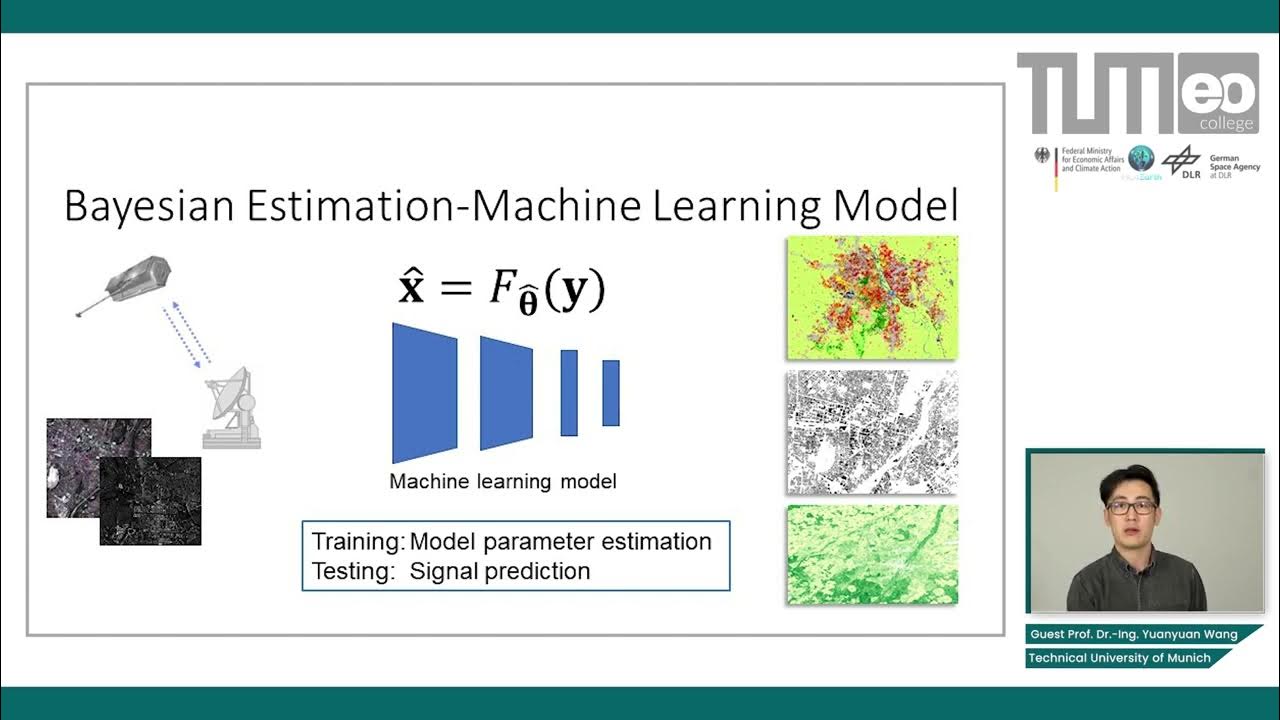
Bayesian Estimation in Machine Learning - Maximum Likelihood and Maximum a Posteriori Estimators
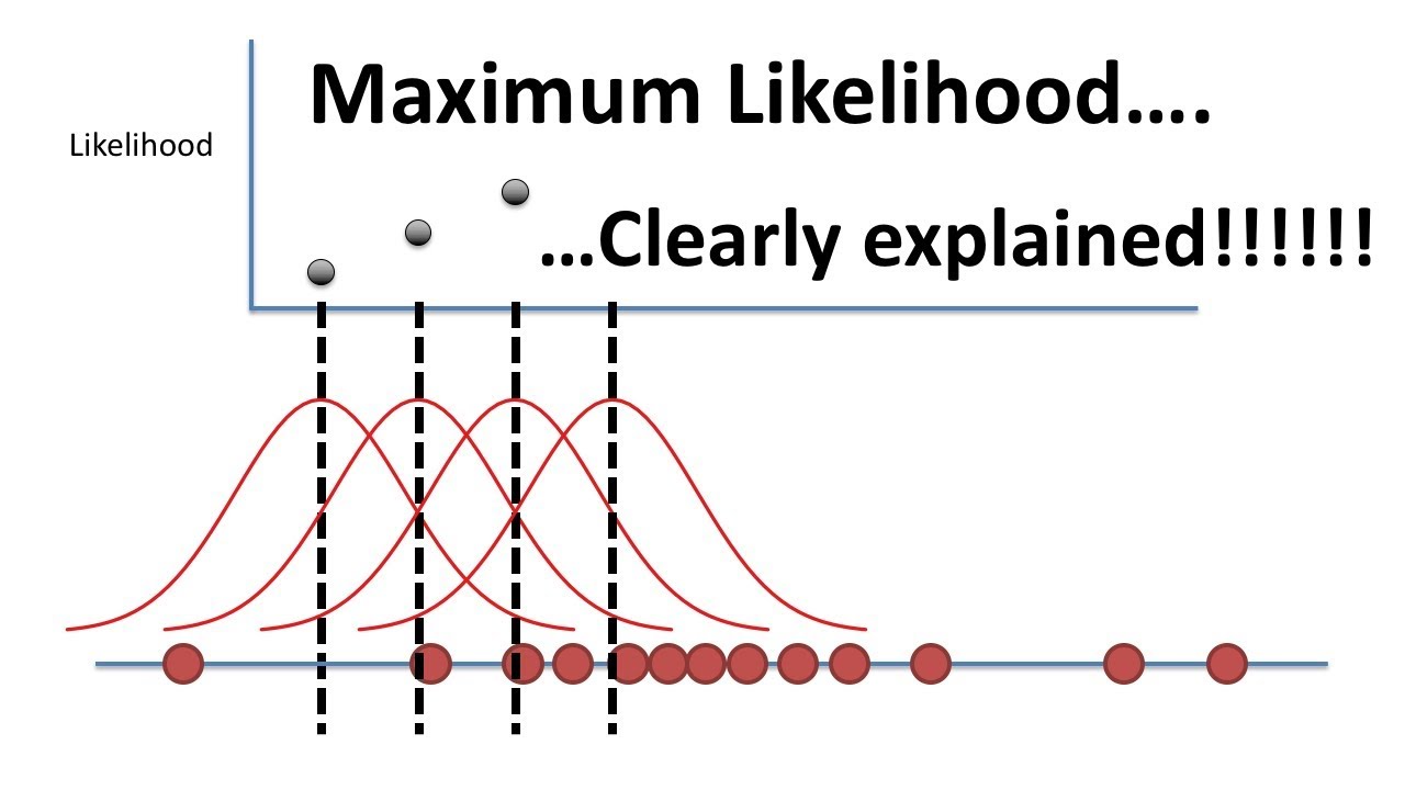
Maximum Likelihood, clearly explained!!!
Presentation16: Using Maximum Likelihood Estimation to Calibrate a Discrete Time Markov Model
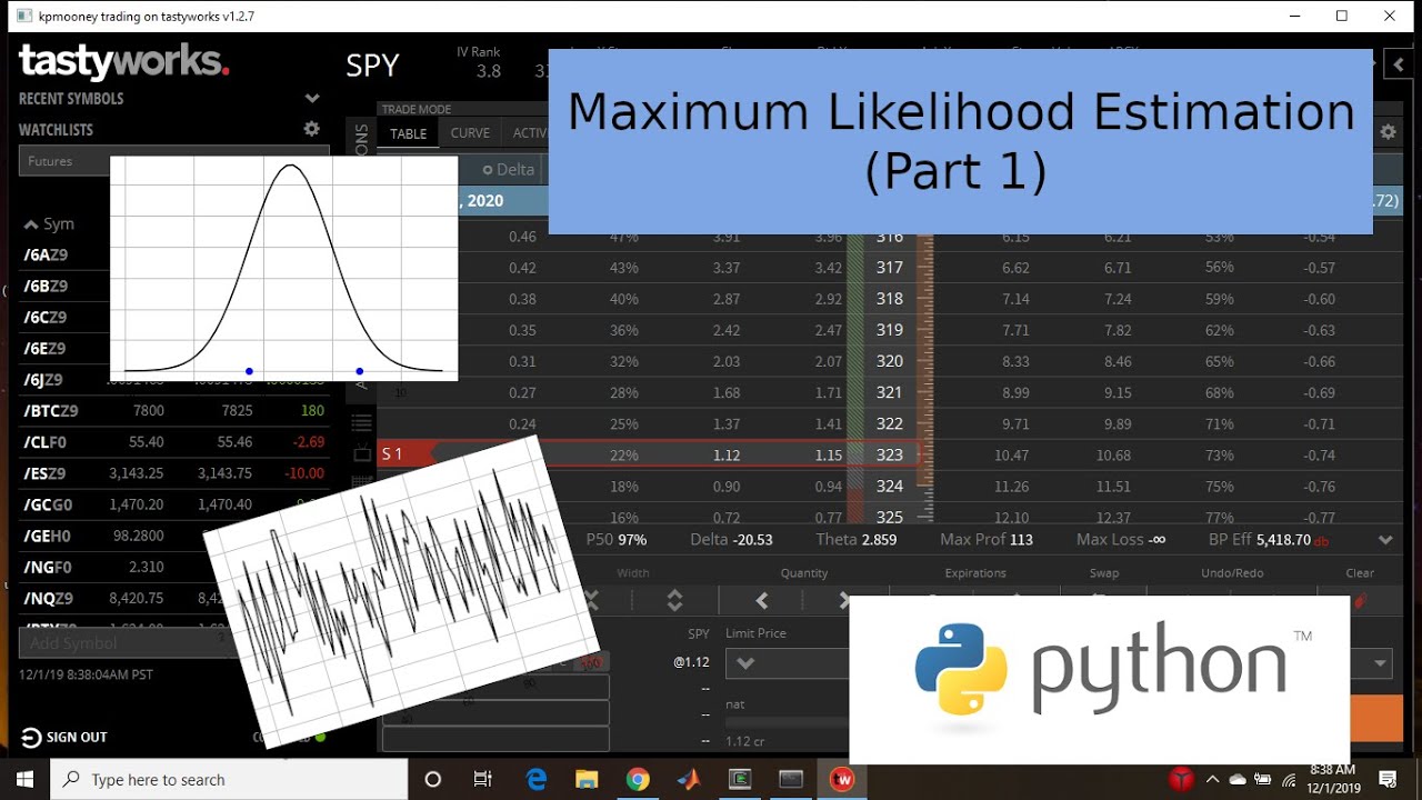
Maximum Likelihood Estimation (Part 1)

Applying MLE for estimating the variance of a time series

Lec-5: Logistic Regression with Simplest & Easiest Example | Machine Learning
5.0 / 5 (0 votes)