Structural Equation Modeling: what is it and what can we use it for? (part 1 of 6)
Summary
TLDRStructural Equation Modeling (SEM) is a comprehensive framework integrating multivariate techniques from various disciplines. It is particularly useful for analyzing complex constructs and relationships, including indirect effects. SEM uses latent variables and path analysis to model causal systems and correct for measurement errors, with software like AMOS and LISREL available for implementation.
Takeaways
- 🔍 Structural Equation Modeling (SEM) is a comprehensive framework that integrates various multivariate techniques from disciplines such as psychology, statistics, and econometrics.
- 📊 SEM is not a single technique but a dynamic modeling environment that evolves to incorporate new ways of fitting models over time.
- 🎯 SEM is particularly suitable for addressing complex research questions involving multifaceted constructs, such as psychological concepts, and for modeling causal systems with multiple outcomes or dependent variables.
- 🔍 SEM is adept at handling indirect or mediated effects, where the effect of one variable on another is transmitted through a third variable.
- 📚 SEM is known by various names, including covariance structure analysis, analysis of moment structures, and LISREL models, reflecting its diverse origins and applications.
- 💻 There are numerous software packages available for SEM, each with its own advantages and disadvantages, and some offer free versions for students to explore.
- 🛣 SEM can be thought of as path analysis using latent variables, which are underlying constructs that influence attitudes and behaviors but are not directly observable.
- 📝 Latent variables are measured using observable indicators, such as questionnaire items, which are believed to be caused by the underlying latent constructs.
- 🔧 SEM employs a true score equation, where the observed variable is comprised of a true score and error, and the goal is to isolate the true score while removing the error variance.
- 📈 The use of multiple indicators for latent constructs in SEM allows for the correction of measurement errors and provides a better estimate of the true score.
- 🔗 Path analysis, a key component of SEM, visually represents models diagrammatically, emphasizing direct, indirect, and total effects in the relationships between variables.
Q & A
What is the primary distinction of Structural Equation Modeling (SEM) compared to other statistical techniques?
-SEM is not a single technique but a general modeling framework that integrates various multivariate techniques into one environment, drawing on disciplines like psychology, statistics, epidemiology, and econometrics.
How does SEM differ from traditional statistical methods in terms of the research questions it can address?
-SEM is particularly suitable for addressing complex research questions involving multifaceted constructs, systems of relationships, causal systems, and indirect or mediated effects, which might be more challenging with traditional statistical methods.
What are some alternative names for SEM found in literature, and why might they be used?
-SEM is also known as covariance structure analysis models, analysis of moment structures, and LISREL models, named after the first software for fitting SEMs. The term causal modeling is sometimes used but is controversial as causality comes from research design, not the statistical model.
What are some of the software packages available for conducting SEM analysis?
-Several software packages are available for SEM, including LISREL, Mplus, EQS, AMOS, CALIS, and R. Each package has its advantages and disadvantages, and some offer free or limited versions for students.
How is SEM defined in terms of path analysis and latent variables?
-SEM can be thought of as path analysis using latent variables, which are hypothetical or not directly observable constructs that are measured using observable indicators.
Why are latent variables important in social science research, and how are they measured?
-Latent variables are important because many social science concepts, like intelligence or trust, are not directly observable. They are measured using observable indicators, such as questionnaire items, which are believed to be caused by the underlying latent constructs.
What is the significance of the true score equation X = t + e in SEM?
-The true score equation represents the idea that the observed variable X is comprised of a true score (t), which is the individual's actual level on the measured construct, and error (e), which includes random and systematic error variance.
Why is it necessary to have multiple indicators for latent constructs in SEM?
-Having multiple indicators is necessary to over-identify the true score equation, allowing for the estimation of true scores and error variance for each indicator, and providing a better measure of the concept by correcting for measurement error.
How does the use of multiple indicators benefit the measurement of latent constructs in SEM?
-Multiple indicators help to capture the complexity of the construct, reduce random error in the measurement, and provide more precise and accurate estimates of the construct, leading to better model estimates and less bias in effect sizes.
What is the role of path analysis in SEM, and how does it differ from traditional regression analysis?
-Path analysis in SEM is used to represent the model diagrammatically, focusing on both direct and indirect effects in the relationships between variables. It differs from traditional regression analysis by providing a visual representation and allowing for the examination of complex causal pathways.
How can indirect effects be identified and calculated in SEM?
-Indirect effects can be identified through path diagrams that show the pathways between variables. They are calculated by multiplying the direct effects along the pathway (e.g., beta2 * beta3 in the example given), and the total effect is the sum of direct and indirect effects.
Outlines

此内容仅限付费用户访问。 请升级后访问。
立即升级Mindmap

此内容仅限付费用户访问。 请升级后访问。
立即升级Keywords

此内容仅限付费用户访问。 请升级后访问。
立即升级Highlights

此内容仅限付费用户访问。 请升级后访问。
立即升级Transcripts

此内容仅限付费用户访问。 请升级后访问。
立即升级浏览更多相关视频

HASIL ANALISIS SEM part 1

part 2, 9nov
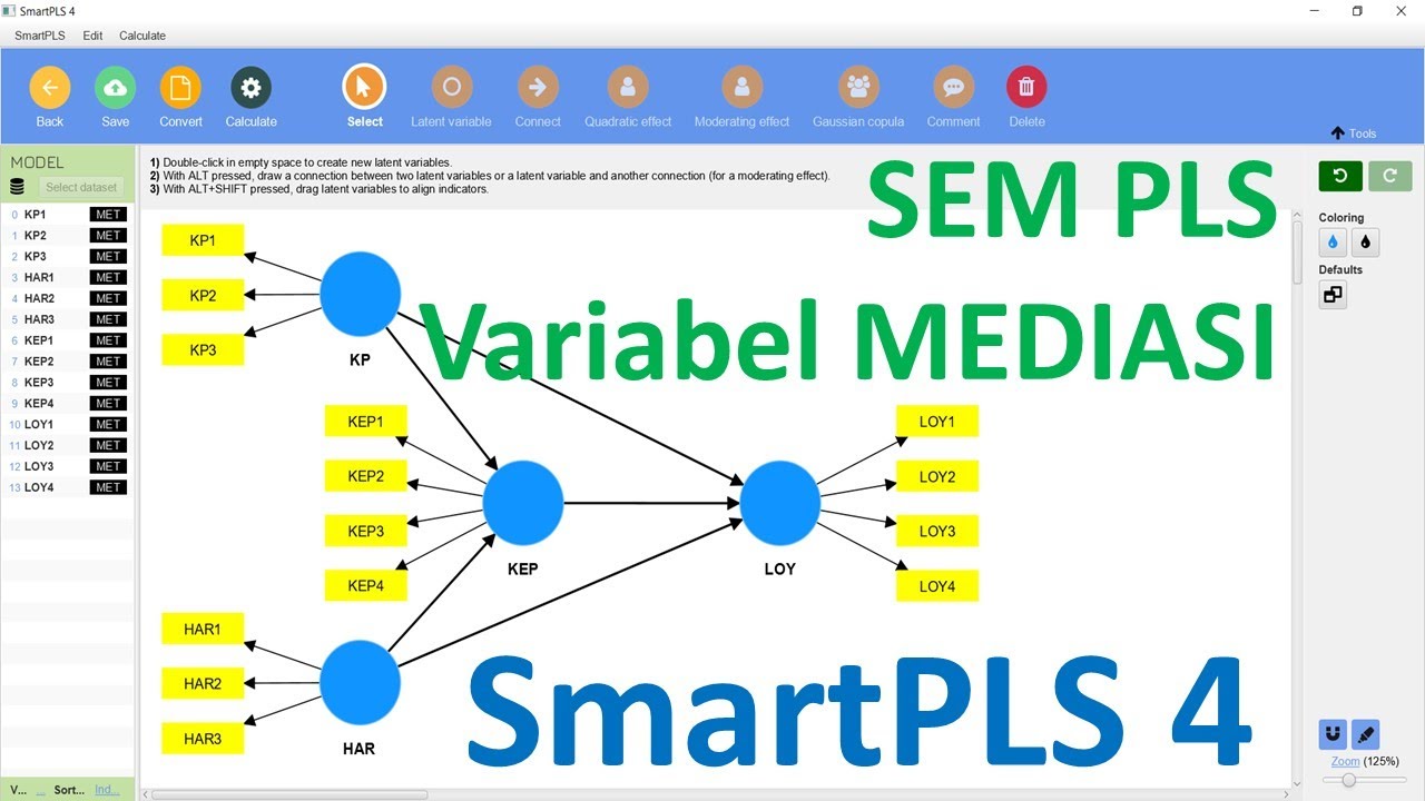
Tutorial SEM PLS dengan Variabel Mediasi Menggunakan SmartPLS 4 || Lengkap dengan referensi
TUTORIAL SMARTPLS 4: CARA MEMBUAT LAPORAN SEM PLS REFERENSI HAIR ET AL, 2022 (TERBARU)

TUTORIAL SEM PLS: METODE ANALISIS DATA

Dr. Arif Jauhar Tontowi - Video Mengenal Alat Analisis SEM - Bengkel Inovasi
5.0 / 5 (0 votes)
