Tutorial Cara Uji Normalitas dengan JASP
Summary
TLDRThis video explains three key methods for testing data normality using statistical software: visual inspection (histogram and boxplot), statistical tests (Kolmogorov-Smirnov and Shapiro-Wilk), and analysis of skewness and kurtosis. The visual method is best for large datasets, while statistical tests are more reliable with moderate sample sizes. Skewness and kurtosis values help determine if the data's distribution is symmetric and bell-shaped. Each method has its limitations, especially with large or small samples. The video emphasizes using a combination of methods for a robust normality check, depending on your data's size and context.
Takeaways
- 😀 Uji normalitas (normality test) can be performed using three methods: visual inspection, statistical tests, and examining skewness and kurtosis.
- 😀 The visual method involves inspecting histograms, Q-Q plots, or boxplots to check for a bell-curve shape, which indicates normal distribution.
- 😀 In the Kolmogorov-Smirnov test, data is considered normal if the p-value is greater than 0.05.
- 😀 The Shapiro-Wilk test also checks for normality, with a p-value greater than 0.05 suggesting that data follows a normal distribution.
- 😀 Skewness and kurtosis can be used to assess normality, with ideal values being close to 0 and within the range of -1.96 to +1.96 for z-scores.
- 😀 Data is considered normally distributed if the histogram is bell-shaped, with most data points clustered around the mean.
- 😀 Q-Q plots can also help identify normality; points closer to the reference line indicate normality.
- 😀 Skewness refers to the asymmetry of the data, while kurtosis indicates how 'peaked' or 'flat' the distribution is.
- 😀 If skewness and kurtosis values fall within the range of -1.96 to +1.96, the data is considered normally distributed.
- 😀 For large sample sizes, statistical tests like Shapiro-Wilk may show significant results even if the data is approximately normal, due to the sensitivity of these tests to large datasets.
- 😀 Visual methods are generally more reliable for larger samples (over 200), while smaller sample sizes may need more caution when interpreting normality using statistical tests.
Q & A
What are the three methods to test for normality in data as discussed in the video?
-The three methods to test for normality in data are: 1) Visual method (using histograms, Q-Q plots, or boxplots), 2) Statistical tests (such as Kolmogorov-Smirnov and Shapiro-Wilk tests), and 3) Skewness and Kurtosis values.
How is normality visually assessed using histograms?
-Normality is assessed visually by observing the shape of the histogram. A normal distribution should resemble a bell curve, where data is concentrated around the mean and tapers off symmetrically as it moves away from the center.
What does the Kolmogorov-Smirnov test measure in terms of normality?
-The Kolmogorov-Smirnov test measures the difference between the sample distribution and the normal distribution. If the p-value is greater than 0.05, the data is considered to be normally distributed.
What is the significance of the Shapiro-Wilk test in normality testing?
-The Shapiro-Wilk test checks the null hypothesis that the data is normally distributed. If the p-value is greater than 0.05, it indicates that the data does not significantly deviate from a normal distribution, hence it is considered normal.
What do skewness and kurtosis values tell us about data distribution?
-Skewness measures the asymmetry of the data distribution. A skewness value close to 0 suggests a symmetric distribution. Kurtosis measures the peak or flatness of the distribution. A kurtosis value close to 0 suggests a normal distribution, with values outside the range of -1.96 to +1.96 indicating deviations from normality.
What is the ideal range for skewness and kurtosis in a normal distribution?
-For a normal distribution, skewness should be between -1 and +1, and kurtosis should ideally be between -1.96 and +1.96.
How do you calculate Z-scores for skewness and kurtosis?
-Z-scores for skewness and kurtosis are calculated by dividing the skewness or kurtosis value by its respective standard error. A Z-score falling within the range of -1.96 to +1.96 indicates normality.
What sample size is recommended for using visual methods to assess normality?
-Visual methods, such as histograms and Q-Q plots, are more effective for large sample sizes (e.g., greater than 200). For smaller samples, statistical tests are preferred.
What is a limitation of using the Shapiro-Wilk test with large sample sizes?
-A limitation of the Shapiro-Wilk test is that with large sample sizes, even small deviations from normality can become statistically significant, leading to a false rejection of the null hypothesis (normality).
Why might skewness and kurtosis not be reliable for small sample sizes?
-For small sample sizes, the standard error of skewness and kurtosis is larger, which can result in skewness and kurtosis values being less reliable for detecting normality. Therefore, it is harder to detect true deviations from normality with small datasets.
Outlines

此内容仅限付费用户访问。 请升级后访问。
立即升级Mindmap

此内容仅限付费用户访问。 请升级后访问。
立即升级Keywords

此内容仅限付费用户访问。 请升级后访问。
立即升级Highlights

此内容仅限付费用户访问。 请升级后访问。
立即升级Transcripts

此内容仅限付费用户访问。 请升级后访问。
立即升级5.0 / 5 (0 votes)

