A "Crash Course" to Spatial Interpolation
Summary
TLDRIn this video, Anastasios Dardis from Ezra Canada explores spatial interpolation in ArcGIS Pro, a technique for estimating values at unsampled locations using geocoded sample points. He explains two main methods: deterministic, which uses mathematical formulas, and geostatistical, employing statistical models with spatial autocorrelation. The tutorial covers popular models like IDW and Kriging, discussing their applications, advantages, and limitations. Dardis also guides viewers through the iterative process of selecting a model, setting parameters, and validating results using cross-validation, ultimately helping users apply spatial interpolation effectively.
Takeaways
- 🌐 Spatial interpolation is a technique used to estimate values at unknown points or areas based on geocoded sample points with known values.
- 📈 It is more efficient and cost-effective to use spatial interpolation to map unknown values at unsampled locations rather than extracting samples at every location.
- 🔍 Spatial interpolation applies Tobler's First Law of Geography, which states that everything is related to everything else, but near things are more related than distant things.
- 💧 It is widely used in various disciplines such as hydrology, soil, agriculture, weather, climate, atmosphere, land use, and topography.
- 🛠️ There are two types of spatial interpolation techniques: deterministic (mathematics-based formulas) and geostatistical (statistical models with spatial autocorrelation).
- 📊 Deterministic methods like IDW provide smooth interpolated surfaces and are easier to understand and process, while geostatistical methods like Kriging are more complex but consider distance and variation between data points.
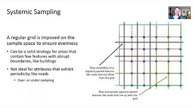
- 📉 IDW is efficient for large datasets and good for high spatial density, but it may not be suitable for small datasets or areas with abrupt changes.
- 🔍 Kriging is excellent for smaller datasets, identifies interpolation errors, and considers spatial autocorrelation, but it can be computationally intensive and requires knowledge of geostatistics.
- 🔄 The process of spatial interpolation is iterative and includes visualizing data, exploring for outliers or skewness, selecting a model, checking its accuracy, and comparing multiple models if necessary.
- 📊 Decision trees developed by ESRI can guide the selection of the most appropriate spatial interpolation model based on various factors such as the type of information required, method complexity, and desired level of smoothness.
- 📈 A semi-variogram is used in geostatistical methods to visualize spatial autocorrelation and help determine parameters such as the sill, range, and nugget effect.
Q & A
What is spatial interpolation?
-Spatial interpolation is a technique that uses geocoded sample points with known values to estimate values at unknown points or areas. It's more efficient and cost-effective than extracting samples at every location.
Why is spatial interpolation important?
-Spatial interpolation is important because it allows for the prediction of values at unsampled locations, which can be costly or impractical to directly measure. It's widely used across various disciplines such as hydrology, soil science, agriculture, weather, and climate.
What is Tobler's First Law of Geography, and how does it relate to spatial interpolation?
-Tobler's First Law of Geography states that 'everything is related to everything else, but near things are more related than distant things.' This law is fundamental to spatial interpolation as it suggests that the value at an unknown location can be estimated based on the values of nearby locations.
What are the two types of techniques used in spatial interpolation?
-The two types of techniques used in spatial interpolation are deterministic and geostatistical. Deterministic methods use mathematical formulas, while geostatistical methods use statistical models that consider spatial autocorrelation.
What is the difference between deterministic and geostatistical methods?
-Deterministic methods, like Inverse Distance Weighting (IDW), assign values based on surrounding measured values, and they are smooth and simple to understand. Geostatistical methods, like Kriging, consider distance and variation between known data points, predict with accuracy, and identify interpolation errors, but they are more complex and computationally intensive.
What are the advantages and disadvantages of IDW?
-IDW is efficient for large datasets, easy to understand, and good for high spatial density. However, it is not suitable for small datasets, assumes similar values for closer points (not good for abrupt changes), and does not consider spatial autocorrelation.
What are the advantages and disadvantages of Kriging?
-Kriging considers distance and variation between data points, is prediction-based, and identifies interpolation errors. It is excellent for smaller datasets. However, it can be complex, requires knowledge of geostatistics, and cannot identify absolute min or max values outside the current range.
What is the role of cross-validation in spatial interpolation?
-Cross-validation is used to check the accuracy of the spatial interpolation model by comparing the predicted values with the actual values. It helps to fine-tune the model parameters and select the best-performing model.
How does the semi-variogram help in spatial interpolation?
-The semi-variogram visualizes spatial autocorrelation and helps in determining the model parameters such as the sill, range, and nugget. It aids in understanding the spatial structure of the data and in fitting the best semi-variogram model to predict values at unsampled locations.
What are the key parameters to consider when performing spatial interpolation?
-Key parameters include lag size, lag tolerance, direction, angle tolerance, bandwidth, and the type of semi-variogram model (e.g., spherical, Gaussian, exponential). These parameters influence how spatial autocorrelation is measured and how values at unknown locations are predicted.
What tools are available in ArcGIS Pro for spatial interpolation?
-ArcGIS Pro offers the Interpolation toolset in the Spatial Analyst toolbox for deterministic methods, the Interpolation toolset in the Geostatistical Analyst toolbox for geostatistical methods, and the Geostatistical Wizard for an interactive approach to spatial interpolation.
Outlines
🌏 Introduction to Spatial Interpolation in ArcGIS Pro
Anastasios Dardis introduces himself as a higher education developer at Ezra Canada and presents the topic of spatial interpolation in ArcGIS Pro. Spatial interpolation is a technique that estimates values at unknown points or areas using geocoded sample points. It is more efficient and cost-effective than extracting samples at every location. The method is based on Tobler's First Law of Geography, which states that everything is related, especially nearby things. Spatial interpolation is widely used in various disciplines such as hydrology, soil science, agriculture, weather, climate, atmosphere, land use, and topography. The video will discuss two types of techniques: deterministic, which uses mathematical formulas, and geostatistical, which uses statistical models with spatial autocorrelation. Deterministic methods are smoother and simpler, while geostatistical methods provide more accuracy but are more complex.
📊 Spatial Interpolation Techniques and Models
The script explains the differences between deterministic and geostatistical methods in spatial interpolation. Deterministic methods, like Inverse Distance Weighting (IDW), Natural Neighbor, Trend, and Spline, assign values based on surrounding measures, are efficient for large datasets, and are aesthetically smooth. Geostatistical methods, such as Kriging, Co-kriging, Empirical Bayesian Kriging (EBK), and others, consider distance and variation, are excellent for smaller datasets, and can identify interpolation errors. The script also mentions that IDW is not suitable for datasets with abrupt changes and does not account for spatial autocorrelation. Kriging, on the other hand, is more complex but can predict and provide accuracy measures. The tutorial will cover IDW and Kriging in detail.
🛠️ Steps and Considerations for Spatial Interpolation
The script outlines the multi-step process of spatial interpolation, which includes visualizing data for patterns or trends, exploring data for outliers or skewness, selecting a spatial interpolation model, filling in required parameters, and checking model accuracy through cross-validation. It emphasizes the importance of understanding data, using decision trees to choose the most appropriate model, and iteratively refining parameters. The tutorial also discusses the concept of semi-variograms, which are used to visualize spatial autocorrelation in geostatistical methods. The script explains how to interpret semi-variograms, including the sill, range, and nugget effect, and how these are influenced by parameters like lag size and tolerance.
📚 Conclusion and Additional Resources
The script concludes by emphasizing the importance of understanding spatial interpolation and the steps involved in the process. It mentions that the tutorial will cover how to apply the concepts learned, perform cross-validation, and identify the best model to use. The video encourages viewers to access additional resources, subscribe to the higher education listserv for updates, and follow on social media for more educational content related to ArcGIS software. The resource finder page is highlighted as a place to find a range of tutorials from ArcGIS Pro to ArcGIS Enterprise.
Mindmap
Keywords
💡Spatial Interpolation
💡Geocoded Sample Points
💡Deterministic Methods
💡Geostatistical Methods
💡Tobler's First Law of Geography
💡Cross-validation
💡Semi-variogram
💡Lag Size
💡Anisotropy
💡Spatial Analyst Toolbox
💡Geostatistical Analyst Toolbox
Highlights
Spatial interpolation is a technique that estimates values at unknown points using geocoded sample points.
Spatial interpolation is more efficient than extracting samples at every location.
It applies Tobler's First Law of Geography, which states that near things are more related than distant things.
Spatial interpolation is widely used in hydrology, soil, agriculture, weather, climate, atmosphere, land use, and topography.
There are two types of spatial interpolation techniques: deterministic and geostatistical.
Deterministic methods use mathematics-based formulas, while geostatistical methods use statistical models with spatial autocorrelation.
Deterministic methods are smooth, whereas geostatistical methods are less so.
Inverse Distance Weighting (IDW) is a popular deterministic method, efficient for large data sets.
Kriging is a geostatistical method that considers distance and variation between known data points.
Kriging identifies interpolation errors, demonstrating the model's performance.
Spatial interpolation is a multi-step and iterative process involving data visualization, exploration, model selection, and validation.
ESRI provides decision trees to help select the most appropriate spatial interpolation model.
Parameters for spatial interpolation models need to be defined through an iterative process of experimentation.
A semi-variogram is used to visualize spatial autocorrelation in geostatistical methods.
The nugget effect is an estimate of error affected by volume sampling and should be minimized.
Lag size, tolerance, and direction are important components in fitting the semi-variogram model.
Cross-validation is used to assess the accuracy of the spatial interpolation model.
ArcGIS Pro offers toolsets for both deterministic and geostatistical spatial interpolation methods.
The Geostatistical Wizard in ArcGIS Pro provides an interactive interface for spatial interpolation.
The resource includes three tutorials for understanding, applying, and validating spatial interpolation models.
Transcripts
hello everyone
my name is anastasios dardis and i'm a
higher education developer at the
education
and research group at ezra canada
in this video you will learn spatial
interpolation in arcgis pro
so what is spatial interpolation
well spatial interpolation is a
technique that uses geocoded sample
points with values to estimate values at
unknown point slash areas the reason
this gis
method exists is it because it is more
efficient to map
unknown values at unsampled locations
than it is to extract samples at every
location
additionally extracting samples at every
location can be quite expensive
to predict values at unknown points
spatial interpolation uses either
deterministic
or geostatistical methods which will be
discussed in the next
slide at its core
spatial interpolation applies tobler's
first law of geography
to identify unknown values at unsampled
areas
for review tobler's first law states
that everything is related to everything
else
but near things are more related than
distant things
thus we could say that spatial
interpolation is widely used across
disciplines
the most popular use cases are in the
fields of hydrology
soil agricultural weather and climate
atmosphere land use and topography
here we can see an image of sample
points in california
collecting ozone levels and then the
next image is interpolating those valves
to display
all of california
in spatial interpolation there are two
types of techniques
deterministic and geostatistical
the differences are the following
backend
deterministic uses mathematics-based
formulas
whereas geostatistical use statistical
models with spatial autocorrelation
what it actually does is that in
deterministic is it assigns
values of locations based on surrounding
measure values
whereas geostatistical predicts and
provides accuracy
as for aesthetics deterministic are
smooth whereas geostatistical are less
so
and both sides have a wide range of
tools to execute
deterministic has inverse distance
weighting or known as idw
natural neighbor trend radial basis
and spline in contrast geostatistical
has
cragging co-creating empirical base
intriguing
or known as ebk ebk regression
ebk 3d and air interpolation
and lastly deterministic are more simple
to understand
and process whereas geostatistical are
not
the next slide shows the concepts
disadvantages
and disadvantages of the most popular
spatial interpolation model
for the sake of time we will go through
idw and kriging
as they will be used in the tutorial
natural neighbor
spline and trend won't be used however
you will have access to this powerpoint
as reference when downloading the
resource from our
higher education page idw
increases its distance decay weight when
a sample location is
relatively close to unknown location
idw is one of the most popular as it is
efficient for large data sets
it's easy to understand and it's good
for high spatial density
however it is not good for small data
sets it assumes that closer points have
similar values
which is not good for abrupt changes
such as mountains and peaks
and is not based on spatial
autocorrelation
on the other hand krigging is somewhat
similar to idw
except it considers distance and the
degree of variation
between known data points
unlike idw trigging is prediction based
has a wide range of methods it's
excellence for smaller data sets
and most importantly it identifies
interpolation errors which demonstrates
the model's performance
the downside of krigging is that it can
be complex
and requires background knowledge of
geostatistics when modeling
it cannot identify values of the
absolute min or max
meaning that values that are higher or
lower than the current range
and lastly kragen can be computationally
intensive
indicating slower processing times
both idw and krigging are thoroughly
discussed in the tutorial in terms of
how they work
now for those of you that are not
familiar with spatial interpolation
it is a multi-step and iterative process
first you visualize the data on the map
and see if there are
any patterns or trends with the data
second
you explore the data and see if there
are any outliers or skewness
if outliers exist you may need to remove
it
if the data is skewed you would have to
perform some data transformation
ignoring these refinement steps could
result in accurate models
next you pick your spatial interpolation
model
fill in required parameters and check
the model's accuracy
by looking at a preview of it and
diagnostic statistics via cross
validation
which is the fifth step ideally
it is best to have at least two models
that way you can compare each of the
model and select the best performing one
now the big question is which model do
you pick
fortunately at esri they have developed
decision trees
as guidance to pinpoint the most
appropriate models
each decision tree asks you a question
and it provides the result
these are what type of information does
your decision require
which method requires measurement or
model spatial
autocorrelation what output type do you
care most
what is the level of assumptions and how
complex do you want your model to be
what type of interpolation you want
what level smoothes do you want would
you like to have
uncertainty of the predicted values and
how fast do you want to interpolate your
model
these are questions you should ask
before starting the interpolation
process
so let's say you've selected your
spatial interpolation models
there are several required parameters
you will have to fill in
unfortunately there is no silver bullet
to properly define the parameters
instead it is an iterative process of
experimentation based on a set of clues
these clues are mining and understanding
your data
checking the model decision tree
checklist
understanding this in my variogram and
deciding the lag size
direction type of model and whether to
combine
multiple models into one that is if it
is applicable
you'll only interpret the semi-varigram
whenever you've decided to use kriging
code kriging or empirical beige
intriguing as your spatial interpolation
model
a semi-varigram is essentially what
visualizes spatial autocorrelation
in case you're not familiar with spatial
autocorrelation
it is a measure of similarity between
nearby observations
in a semi-varigram you have to look at
when the model flattens out
or in other words when spatial
autocorrelation
ceases to exist by identifying three
components
the first is the sill which is the
maximum value or semi-variance
the second is the range which is the
maximum distance reached
and the third is a nugget the nugget is
the value at which the semi-varigram is
virtually close to the y
value here is an image of what it would
look like
the nugget effect is an estimate of
error affected by volume sampling
if the nugget is relatively high from
zero it implies of a large nugget effect
which is something to avoid having in
the model if possible
if you do have a large nugget effect
then there could be measurement
inaccuracies
regards the predictions at unsampled
locations
or spatial sources of variation at
distances smaller than the sampling
interval
in other words it is unpredictable over
very short distances
that is why it is colloquially phrased
as a nugget effect
when gold miners come across a gold
nugget in soils with very low
concentrations of gold
the best way to reduce the nugget effect
is to increase the number of samples
especially at closer intervals
the sill range and nugget are impacted
by several model parameters
the first is lag size that defines the
increment distance intervals
to measure spatial autocorrelation
determining a lag size cannot be too
large as it would skip
short range spatial autocorrelation
neither too small
as it may not represent enough
information
the rule of thumb is to take half of the
largest distance among all points
divided by the number of lags
for example the largest distance between
two sample points
is a hundred kilometers and you want to
set the number of lags to ten
the lag size would be set to five
kilometers another way is to execute
average nearest neighbor tool in arcgis
pro and take the observed mean distance
if your sample happens to be clustered
then go for a smaller number than the
observed mean distance value
next which is not required but may
improve the model's performance
is lag tolerance this is the tolerance
range between lags
usually at half the lag size which
captures extra sample points
increase the lag tolerance only if the
semi-varigram seems to be erratic
another important component is the
direction
this is only used when you see a
directional pattern or influence in the
data
hence the term anisotropy if
anisotropy exists in the data then set
the angle tolerance which is
conceptually
similar to electron tolerance and the
bandwidth
which is the maximum search width to
include other sample points
the next is fitting the calculated semi
variances across the log distance
which is then used to predict data
values at unsampled locations
in arcgis pro there are many such as k
bessel
j bessel hall effect pentospherical and
tetrospherical
however the most popular ones are
spherical
gaussian and exponential given their
simplicity and robustness
lastly is combining multiple fitting
models into one
this is only to be used if you have
other variables that would influence the
phenomena
such as elevation for temperature or
biomass here are two images of what the
parameters would look like if you were
to do this on paper
and on the map
in the final step of modeling you would
assess
the the blue line are known as a
semi-varigram model
the question is does the semi-varigram
model pass through the center of the
cloud of bin values
which are the red dots does it pass as
closely as possible to the average
values which are the blue crosses
and does it pass as closely as possible
through the middle of the local
polynomials displayed as green lines
if the answer is yes to all of them then
you can assess the final part of
modeling via cross validation
cross validation contains the the
statistic diagnostics
these include asking the whether the
regression line displayed as blue
is closely aligned with the reference
gray line
are the points closely lined with a
normal qq plot line
is the mean prediction error close to
zero
is the root mean square as small as
possible
and is the average standard error
similar to the root mean square
if you're using ebk based methods
further questions you need to ask is
whether the 90
interval is close to 90 the 95 percent
interval is close to 95
and the average continuous rank
probability score
is as small as possible if most of your
results are within these guidelines
then the model likely perform well and
can be exported
in arcgis pro there are several tool
sets that can be used to execute spatial
interpolation models
the first is the interpolation toolset
located in the spatial analyst toolbox
this is more mathematical based on value
and distance and is not interactive
the other is the interpolation toolset
located in the geostatistical analyst
toolbox
this one is strictly for the
geostatistical methods
and finally the geostatistical wizard
which has the
most of the spatial interpolation
methods this graphical user interface
is powerful as it is interactive and
provides previews of the interpolated
surface before exporting
you will use this one in this tutorial
finally when you download the resource
it will consider a set of three
tutorials
see how it is structured in the folder
part one is to have a deeper
understanding of spatial interpolation
which is an expansion of the video you
are watching now
and i highly recommend you to go through
this one first
part two is applying of what you've
learned in part one
by probably using the inverse distance
weighting
krigging and empirical bayesian creating
to spatially interpolate air temperature
in the province of new brunswick
and part three is to perform
cross validation and validation to
identify which model
is best to use
thank you for watching the spatial
interpolation resource
if you're a student please subscribe to
our higher education listserv
where you can receive weekly updates
regards to educational resources
using arcgis software if you're not a
student you can still follow us on
at gis ajd lastly
if you'd like to learn more check out
our higher education
resource finder page and there you will
find a range of tutorials from arcgis
pro
to arcgis enterprise
浏览更多相关视频
Spatial Sampling & Interpolation
[S1E6] Cross-Validation | 5 Minutes With Ingo
Python Pandas Tutorial 5: Handle Missing Data: fillna, dropna, interpolate
How to Make Ai Influencer | Ai Influencer kaise banaye 2024
Teori Gravitasi, Titik Henti, dan Grafik | Materi Geografi Kelas XII IPS SMA
Logit model explained: regression with binary variables (Excel)
5.0 / 5 (0 votes)