Vivado HLS Example: FFT
Summary
TLDRThis video script outlines the process of implementing a Fast Fourier Transform (FFT) using Vivado High-Level Synthesis (HLS) tools. It covers generating reference data, writing C code, simulating, synthesizing, and packaging the IP for export. The tutorial skips optimization for simplicity and assumes a Linux environment. It also uses Python for data generation and Anaconda for numeric libraries, emphasizing the importance of experimentation and adaptability across different platforms.
Takeaways
- 📚 The video demonstrates an implementation of the Fast Fourier Transform (FFT) using Vivado HLS tools.
- 🔍 It covers the steps from generating reference data to exporting the IP for use in Vivado tools, excluding optimization topics.
- 🌐 Reference websites are provided for the source code and additional tools like the Anaconda distribution for Python.
- 💻 The demonstration is conducted on a Linux system, but the principles are general and can be adapted to other systems.
- 📝 The process begins by cloning a repository containing all the source code and data for the FFT example.
- 🔢 Data for testing is generated using a Python script that creates random complex values, computes an FFT, and stores the results in different formats.
- 🛠️ The Vivado HLS project is set up with the main source code and test bench, including the generated .txt files for input and expected output.
- 🔄 The part number for the FPGA board is selected to match the hardware that will be used for implementation.
- 🔍 A C simulation is run to ensure the correctness of the implementation before proceeding to synthesis.
- 📈 Post-synthesis RTL co-simulation is performed to confirm that the synthesized design matches the C simulation results.
- 📦 Finally, the RTL is exported as a package for implementation on an FPGA, concluding the design process.
Q & A
What is the main topic of the video?
-The video is about implementing a simple design, specifically the Fast Fourier Transform (FFT), using Vivado High-Level Synthesis (HLS) tools.
What are the steps followed in the video for implementing the FFT design?
-The steps are: 1) Generate reference data for testing, 2) Write C code, 3) Simulate using Vivado HLS, 4) Synthesize and simulate post-synthesis, 5) Package the IP for export and use in Vivado tools for implementation.
Why are certain topics not covered in the video?
-The video does not cover optimization of bit widths, data representations, or design optimization for size, speed, or other metrics to focus on the basic principles of using Vivado HLS tools.
What is the source code of the demonstration available at?
-The source code is available at the website 'get-lab.com/Chandra/children/each-FPGA'.
What is the example used in the video for demonstrating the FFT using HLS?
-The example used is an FFT implementation with HLS, and the audience is encouraged to clone and modify the information from the provided website.
Which Python libraries are mentioned for data analysis and signal processing?
-The video mentions the use of numeric Python libraries, specifically the Anaconda distribution, which includes scientific Python and other libraries useful for data analysis and signal processing.
Is the video's demonstration platform-specific?
-The demonstration is done on a Linux system, but the principles involved are general and can be applied to Windows systems or different Linux distributions with appropriate modifications.
What is the purpose of the 'data_gen_FFT.py' script mentioned in the video?
-The 'data_gen_FFT.py' script generates random input data, computes an FFT, and stores the input and output data in both floating-point and 16-bit fixed-point hexadecimal formats for testing.
What is the significance of the tolerance limit set in the test bench?
-The tolerance limit is set to account for small errors that may occur due to the conversion from floating-point to fixed-point, ensuring the system does not flag an error for minor discrepancies.
What does the synthesis report provide after running C synthesis in Vivado HLS?
-The synthesis report provides information on the target clock period, estimated clock period achieved, latency, initiation interval, and resource usage of the synthesized FFT function.
What is the purpose of running RTL co-simulation after synthesis?
-The RTL co-simulation is run to verify that the synthesized design produces the same results as the C simulation and to observe internal signals and the behavior of the design at the RTL level.
How does the video conclude?
-The video concludes by demonstrating the export of the RTL as a package for implementation on an FPGA in Vivado, marking the end of the design process discussed.
Outlines

This section is available to paid users only. Please upgrade to access this part.
Upgrade NowMindmap

This section is available to paid users only. Please upgrade to access this part.
Upgrade NowKeywords

This section is available to paid users only. Please upgrade to access this part.
Upgrade NowHighlights

This section is available to paid users only. Please upgrade to access this part.
Upgrade NowTranscripts

This section is available to paid users only. Please upgrade to access this part.
Upgrade NowBrowse More Related Video
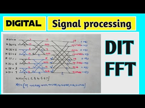
DIT FFT | 8 point | Butterfly diagram

DSP#44 problem on 8 point DFT using DIT FFT in digital signal processing || EC Academy

The Discrete Fourier Transform (DFT)
Understanding the Discrete Fourier Transform and the FFT

Relation between Laplace transform, Fourier transform, z-transform, DTFT, DFT and FFT
The Fast Fourier Transform (FFT)
5.0 / 5 (0 votes)