Statistics for Psychology

Summary

This video script offers an informative overview of the normal distribution, a fundamental concept in statistics. It explains the characteristics of a normal distribution curve, including symmetry, the mean, median, and mode aligning at the center, and its asymptotic nature. The script delves into the significance of the mean and standard deviation, illustrating how they define the spread of data points. It also covers the '68-95-99.7' empirical rule, which quantifies the proportion of data within one, two, or three standard deviations from the mean. The presenter uses the example of gummy bear consumption to demonstrate how to calculate and interpret z-scores, providing a practical application of normal distribution in real-world scenarios.

Takeaways

• 📚 The normal distribution is a fundamental concept in statistics, characterized by its bell shape and symmetry.
• 🔍 The mean, median, and mode of a normal distribution all coincide at the center of the distribution curve.
• 📉 The normal distribution is asymptotic, meaning it extends indefinitely in both directions without ever reaching zero.
• 🌐 The distribution is useful for modeling real-world phenomena because it captures the majority of data within a few standard deviations from the mean.
• 📈 The probability of data points falling within one standard deviation from the mean is approximately 68%, two standard deviations capture about 95%, and three standard deviations nearly 100%.
• 📊 Normal distributions can vary in their means and standard deviations, but the key property of capturing a certain percentage of data within specific standard deviations remains consistent.
• 🔢 The mean represents the average value, while the standard deviation measures the spread or dispersion of the data around the mean.
• 🤔 Understanding the standard deviation helps in gauging how typical a data point is; for example, a person eating 100 pounds of gummy bears per day with a standard deviation of 10 would be considered normal.
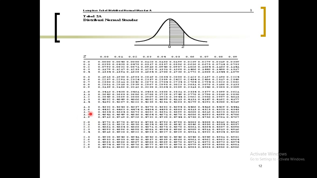
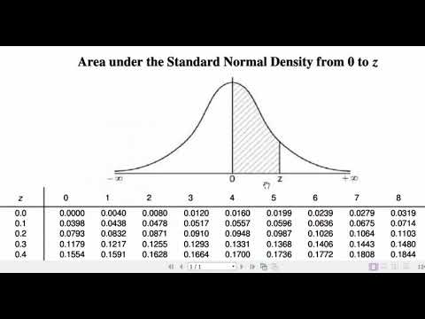
• 📚 To work with different normal distributions, z-scores are used to standardize the data, making it easier to compare and interpret using a single table.
• ➗ The z-score is calculated by subtracting the mean from the data point and then dividing by the standard deviation, indicating how many standard deviations away from the mean the data point lies.
• 🔎 By using z-scores and referring to a standard normal distribution table, one can determine the probability of a data point occurring beyond a certain threshold, like the likelihood of someone eating more than 140 pounds of gummy bears per day.

Q & A

What is the shape of a normal distribution curve?

The normal distribution curve is bell-shaped, symmetrical around its mean, with the mean, median, and mode all coinciding at the center of the curve.

Why is the normal distribution considered to be asymptotic?

The normal distribution is considered asymptotic because it theoretically extends indefinitely in both directions without ever reaching zero, although for practical purposes, it captures nearly all data within a few standard deviations from the mean.

What is the significance of the mean, median, and mode being equal in a normal distribution?

The equality of the mean, median, and mode in a normal distribution signifies that the data is perfectly symmetrical, and the central tendency measures are consistent, reflecting a balanced distribution of data points around the center.

How does the normal distribution help in modeling real-world phenomena?

The normal distribution is useful for modeling real-world phenomena because it captures the central limit theorem, where the sum of a large number of independent and identically distributed variables tends to form a normal distribution, making it a common statistical model for various natural and social phenomena.

What is the Empirical Rule in relation to the normal distribution?

The Empirical Rule states that for a normal distribution, approximately 68% of the data falls within one standard deviation of the mean, 95% within two standard deviations, and 99.7% within three standard deviations.

What is a z-score and how is it calculated?

A z-score is a measure of how many standard deviations an element is from the mean in a normal distribution. It is calculated by subtracting the mean from the data point and then dividing by the standard deviation.

Why is standardizing scores into z-scores useful in statistics?

Standardizing scores into z-scores is useful because it allows for easy comparison of data across different normal distributions, as it transforms the data into a common scale where the mean is 0 and the standard deviation is 1, facilitating the use of standard tables for probability calculations.

What is the relationship between a z-score and the probability of a data point occurring?

The z-score indicates the number of standard deviations a data point is from the mean, and by looking up the z-score in a standard normal distribution table, one can determine the probability or percentage of data points occurring at that distance from the mean.

How can you find the probability of a data point being beyond a certain value in a normal distribution?

To find the probability of a data point being beyond a certain value, calculate the z-score for that value, look up the corresponding area in a standard normal distribution table, and then subtract this area from 0.5 if you want the probability beyond that value in one tail, or from 1 if considering both tails.

What is an example of a practical scenario where the normal distribution is applied as described in the script?

An example given in the script is determining the likelihood of a person eating more than 140 pounds of gummy bears per day, assuming the average consumption is 100 pounds with a standard deviation of 10, by calculating the z-score for 140 and using a standard normal distribution table to find the probability.

How does the script illustrate the concept of 'freakishly high' or 'freakishly low' in the context of the normal distribution?

The script uses the phrase 'freakishly high' or 'freakishly low' to describe data points that are more than one standard deviation above or below the mean, indicating that these occurrences are less common and deviate significantly from the norm.

Outlines

00:00

📊 Introduction to the Normal Distribution

The speaker introduces the concept of the normal distribution, highlighting its importance and common characteristics. They explain that the normal distribution is symmetrical, with the mean, median, and mode all located at the center. The concept of asymptotic behavior is also mentioned, where the curve never touches the x-axis. The speaker emphasizes the practical relevance of the normal distribution in modeling various phenomena.

05:02

📐 Standard Deviation and the 68-95-99.7 Rule

The speaker explains the properties of the normal distribution related to standard deviations. They describe how moving one standard deviation away from the mean captures about 68% of the data, two standard deviations capture about 95%, and three standard deviations capture almost all of the data (99.7%). This section underscores the utility of the normal distribution in understanding data spread and probabilities.

🍬 Applying the Normal Distribution: Gummy Bears Example

A practical example involving gummy bear consumption is used to illustrate the application of the normal distribution. The speaker sets up a problem where the mean consumption is 100 pounds per day with a standard deviation of 10 pounds. They discuss how to calculate the probability of randomly selecting someone who eats more than 140 pounds of gummy bears per day by converting this problem into a z-score and looking up the corresponding probability.

🔢 Understanding and Using Z-Scores

The concept of z-scores is introduced as a method to standardize scores from different normal distributions. The speaker explains how to convert raw scores into z-scores, which represent the number of standard deviations a data point is from the mean. The utility of z-scores in simplifying the lookup of probabilities using standard tables is discussed, along with an example calculation involving a score of 140.

📈 Calculating Probabilities Using Z-Scores

The speaker demonstrates the procedure for calculating probabilities using z-scores. They explain how to look up z-scores in tables and interpret the results. An example is provided where a z-score of +4 is used to find the probability of consuming more than 140 pounds of gummy bears per day. The speaker discusses different types of tables and how to adjust calculations based on the provided data.

📝 Recap and Procedure for Calculating Z-Scores

A summary of the steps involved in calculating z-scores is provided. The speaker reiterates the process: subtracting the mean from the raw score and then dividing by the standard deviation. This section serves as a concise recap of the key points discussed throughout the video, emphasizing the practical application of the normal distribution and z-scores in statistical analysis.

Keywords

💡Normal Distribution

Normal distribution, also known as Gaussian distribution, is a probability distribution that is characterized by its symmetric bell-shaped curve. In the video, it is explained as a fundamental concept for understanding statistical concepts. The mean, median, and mode all coincide at the center of this distribution, which is a key feature used to describe data that follows a normal distribution pattern. The script uses the normal distribution to discuss the likelihood of certain outcomes, such as eating a certain amount of gummy bears.

💡Mean

The mean, often referred to as the average, is a measure of central tendency in statistics. It is calculated by summing all the values in a data set and then dividing by the number of values. In the context of the video, the mean is the central point of the normal distribution where the average value lies, and it is used as a reference point to calculate deviations in the data.

💡Median

The median is another measure of central tendency, representing the middle value of a data set when it is ordered from least to greatest. In the video, it is mentioned that in a normal distribution, the median coincides with the mean, indicating that half of the data lies above and half below this central value.

💡Mode

The mode is the value that appears most frequently in a data set. In the video, it is noted that in a normal distribution, the mode also coincides with the mean and median, meaning the most common value is at the center of the distribution.

💡Standard Deviation

Standard deviation is a measure of the amount of variation or dispersion in a set of values. It indicates how much individual data points in the set typically deviate from the mean. In the video, standard deviation is used to describe the spread of the normal distribution and to calculate z-scores, which are essential for determining the likelihood of certain events.

💡Asymptotic

Asymptotic refers to a property of a function or curve that approaches a certain value or line but never actually reaches it. In the script, it is mentioned that the normal distribution is asymptotic, meaning it extends indefinitely without ever touching the x-axis, which is used to illustrate the behavior of data that is far from the mean.

💡Z-Score

A z-score is a standard score that indicates how many standard deviations an element is from the mean. In the video, z-scores are used to standardize the data from different normal distributions, allowing for the use of a single table to determine probabilities associated with different scores.

💡Sigma (Σ)

Sigma is the Greek letter used to represent the standard deviation in statistics. In the video, 'Sigma' is used to denote the standard deviation when discussing the properties of the normal distribution and when calculating z-scores.

💡Empirical Rule

The empirical rule, also known as the 68-95-99.7 rule, is a shorthand used to remember the percentage of values that lie within one, two, and three standard deviations from the mean in a normal distribution. The video uses this rule to explain the probabilities associated with different ranges of data, such as the likelihood of eating more than 140 pounds of gummy bears.

💡Frequency Distribution

Frequency distribution is a way to summarize data by showing the number of occurrences of each value or range of values in a data set. In the video, the concept is used to describe how data is organized and visualized in a normal distribution, with the frequency of certain outcomes like eating a specific amount of gummy bears.

💡Probability

Probability is a measure of the likelihood that a particular event will occur, often expressed as a number between 0 and 1. In the video, probability is discussed in the context of the normal distribution to determine the likelihood of rare events, such as consuming an unusually high amount of gummy bears.

Highlights

Introduction to the normal distribution and its importance in statistical analysis.

Explanation of the bell curve shape of the normal distribution and its properties.

The mean, median, and mode all coincide in a normal distribution, indicating symmetry.

Asymptotic nature of the normal distribution and its implications for modeling real-world phenomena.

The practicality of the normal distribution in modeling despite its asymptotic behavior.

Understanding the 68-95-99.7 empirical rule for standard deviations in a normal distribution.

The role of the mean as the central value in a normal distribution.

Clarification of the standard deviation as a measure of spread in the data.

Intuitive understanding of standard deviation in relation to the mean.

The concept of 'normal' in the context of standard deviations from the mean.

Illustration of the distribution of gummy bear consumption as an example of a normal distribution.

Procedure for calculating the likelihood of a random individual consuming an unusual amount of gummy bears.

The process of standardizing scores into z-scores for easier comparison across different normal distributions.

Explanation of z-scores as a way to express how many standard deviations a score is from the mean.

Using z-scores to find the probability of a score occurring in a normal distribution.

How to look up z-scores in a standard normal distribution table to find the area under the curve.

Adjusting the area found in the table to find the exact probability for a given score.

General procedure for converting a raw score to a z-score and using it to find probabilities.

Transcripts

[Music]

so what are you guys hi guys so before

we can get start with anything we need

to understand a little bit about the

normal distribution so um let me talk

briefly about it although you probably

already seen this I mean from the last

midterm it is good to talk briefly about

it just to roll up to speed

no.1 distribution looks kind of like

this bow not this bad but kind of like

this okay

and you know the mean the population

mean sits right here so the average sits

right there but also the median the mode

also sit right here so a couple things

you have the mean is equal to the median

is equal to the mode okay the second

thing is he's pretty symmetric so if you

look at this guy he's symmetric and you

can kind of seen on the pictures say for

the fact that I kind of messed it up but

number three is of course he's on

asymptotic this one's not so big a deal

all it means is this guy just keeps

going on and on forever and never quite

flatlines at zero okay so you might be

thinking something like so what good is

that gonna do us right cuz how many

things are asymptotic like things we're

gonna model they're not gonna go

infinitely high and implement low right

but for all effective purposes once you

get outside of 300 deviations above and

below the mean you've pretty much gotten

this entire curve so in that sense the

normal distribution is good okay it's

going to model a lot of things really

really well and we'll see it is the

distribution to go to in a second okay

but first how do I use this sucker so

these are normal distributions have

different means and different standard

deviations right but they all have this

property that when you look at the mean

if you go out one standard deviation to

the right or to the left you'll always

capture basically 60% of this curve some

props have you learned memorize that

some don't if you go out to standard

deviations so two Sigma

right then you're gonna capture about

95% okay and if you go out three like we

said get pretty much everything I think

you get like ninety nine point seven

okay and that's four three standard

deviations so three sigma okay so I

don't wanna spend too much time in this

since you solve this on your last

midterm but we should talk to me and of

course represents the population mean so

this is the average in this standard

sense of the word right and Sigma the

standard deviation that represents how

far from the average is a guy on average

okay so how far from the average are you

on average so it's a measure of spread

okay okay so what's that kinda mean

intuitively let's say the meanest a

hundred and let's say the standard

deviation is like ten that means if you

pick somebody random it's not that

unusual to find someone between say 100

and 110 and it's not that unusual find

someone between say 90 and 100 so you

can go up and down by a standard

deviation and you're kind of average in

a sense okay are pretty normal okay

beyond that then you start to get a

little freakishly high or a little

freakishly low and all that good stuff

okay okay it's no big deal so I get it

the average is the average the standard

deviation is generally how spread out

guys are if you're within a standard

deviation you're pretty quote normal

whatever that means right and if you're

more than one standard deviation above

or more than one standard deviation

below then you're starting to get like a

little freakishly high or freakishly low

okay so no big deal okay so um good then

let's do a problem with this again I'm

gonna do it kind of quickly because I've

seen from the previous midterm you're

comfortable with this but just in case

okay

so let's say you've got a standard

deviation where the average eats 100

pounds of gummy bears per day okay and

let's say for example like the standard

deviation is 10 okay so that means most

people out there will eat between 90 to

110 pounds gummy bears per day okay and

I want to know what's the likelihood you

pick somebody at random and that person

eats more than so let's say more than

let's say 140 pounds of gummy bears okay

so I don't know what's the likelihood

that you pick somebody at random from

the population and you find that they

eat more than 140 pounds of gummy bears

per day okay okay so what's the set up

as always we'll draw in that average

here for 100 right okay remember this is

a frequency distribution so you line up

all the different possible scores and

technically you're going on the

population you're asking people how many

pounds gummy bears do you eat right and

if a bunch of people get 100 then they

get a high mark over here and if not so

many people you'd a 150 pounds of gummy

bears per day then they're kind of over

here

you know the mark 4 that's low okay no

big deal okay so let's try that so first

thing I do is you can talk about numbers

right but this would suck because if I

had a different normal distribution I'd

have a different mean a different

standard deviation I have to look each

one of these guys up and I'd have to

have a separate table for each and

that's really a pain in the butt so what

I want to do instead is we want to what

we want to do is we want to standardize

it so it's a standardized it what you do

is you take this guy and you convert the

actual scores into something called

z-scores

this is just for archimedes z-scores are

a nice nice way of converting these

scores we could use just one table to

figure things out okay and you know that

kind of makes sense because remember the

defining property of the normal curve in

a way is the fact that once you get one

standard deviation above and below you

always hit that same percentage like 68%

okay and if you go to you always hit 95

cetera cetera okay so let's do that so

how do I what's a z-score mean so you

guys remember represents the number of

standard deviations above or below the

mean your score is so the first thing I

do is convert so if you look at that 140

right I want to know how many standard

deviations above or below the mean is

140 so the first thing is I take 140 and

have subtract 100 for a minute everybody

agrees so let's just plot it down here

so here's 140 and we know it's here and

we know this difference is 40 and that's

what we got right but let's say you had

24 eggs and I wanted to know how many

dozen you have if that's the case you

would take your 24 eggs you divide by

the number in a dozen to say you have

two dozen

same thing right so over here you've got

40 points of difference but I want to

know how many standard deviations fit in

there so you look at your 40 points and

you divide by the number of points in

the standard deviation or to be

ten and that would give you four well

that makes sense right is your forty

points above the mean right

but each standard deviation is worth ten

points so if you're forty points above

and each standard deviations worth ten

you really are four standard deviations

above the mean so that's what a z-score

represents so if you had a z-score of

say plus four that means you are four

standard deviations above the mean if

you had a z-score say like negative two

that would mean you're two standard

deviations below the mean okay so this

number that we ended up with is

ridiculously high but that's fine we can

go with that so we now have a z-score is

plus four okay we get a couple of tricks

depending on the sort of table your book

uses you got to remember the fact that

the entire curve is 100% and half the

curve is of course 50% and you can use

tricks for example some books are really

nice once we look up the z-score and we

convert the z-score to plus four right

so that's origines score then you can

look this up in a table or just two high

number but let's pretend let's pretend

for is actually in your book then it

would go here maybe I would draw all

this right if it gives the area of this

shaded region or the percentage for this

shaded region then we're good so if this

were like for example make up a fake

number point zero zero one like that

totally fake number but let's say that's

what the table gave you then that's the

prickly hood that you're going to get a

score 140 or more and that's what we

want okay

however if your table didn't give you

this but only gave you this and let's

say this was something like point four

nine nine like that right then you would

know 140 to a hundred well to the mean

would be point four nine nine but you

want 140 and up and you agree the whole

thing over here is 50%

so that would be 0.5 0 0 minus 0.49 9

which would be point zero zero one okay

just talking about you know you might

have to make minor adjustments depending

on the sort of table they give you but

the procedures still the same take your

score convert it to a z-score look up

that z-score value in the table and then

use whatever they give you the table to

figure out your answer okay so let me

outline the general procedure again all

the way you can run it backwards but

since I feel like most people are

probably comfortable at this you don't

want to take the back will do a poem

with this in a second okay but first

let's remember the procedure my dad I

should have written this out last time

least I'm doing it now remember the

general procedure

z-score you took your score you

subtracted the mean right so remember

before we had 140 we subtracted the mean

is a hundred and then we divided by the

number of points in a standard deviation

so that's a general procedure for

getting the z-score okay