Cell Referencing in Excel (When to add a $ in a cell)

Summary

This video tutorial explains the correct use of dollar signs in Excel formulas, helping users master absolute and relative cell referencing. The presenter goes through five examples, from basic to advanced, demonstrating how to lock rows, columns, or both. By the end of the video, viewers will understand how to handle references correctly in Excel, preventing common formula errors. The video also introduces chart templates and an index-match formula for more complex scenarios, offering downloadable resources to follow along.

Takeaways

• 😌 Understanding where to place dollar signs in Excel formulas is crucial for accurate cell referencing.
• 📈 The tutorial covers five examples that progress from simple to complex, teaching the correct use of dollar signs for both absolute and relative cell references.
• 💾 A free Excel file is provided for practice, which includes the examples discussed in the video.
• 🔄 In the first example, the dollar sign is used to lock the sales tax percentage to a specific cell, ensuring it remains constant when the formula is copied down.
• 🌐 For scenarios with varying tax rates, the dollar sign is strategically placed to lock the tax rate to a specific column while allowing the row to adjust.
• 📊 The tutorial suggests using chart templates from Hotspot to visualize data, which can be automatically updated as data changes.
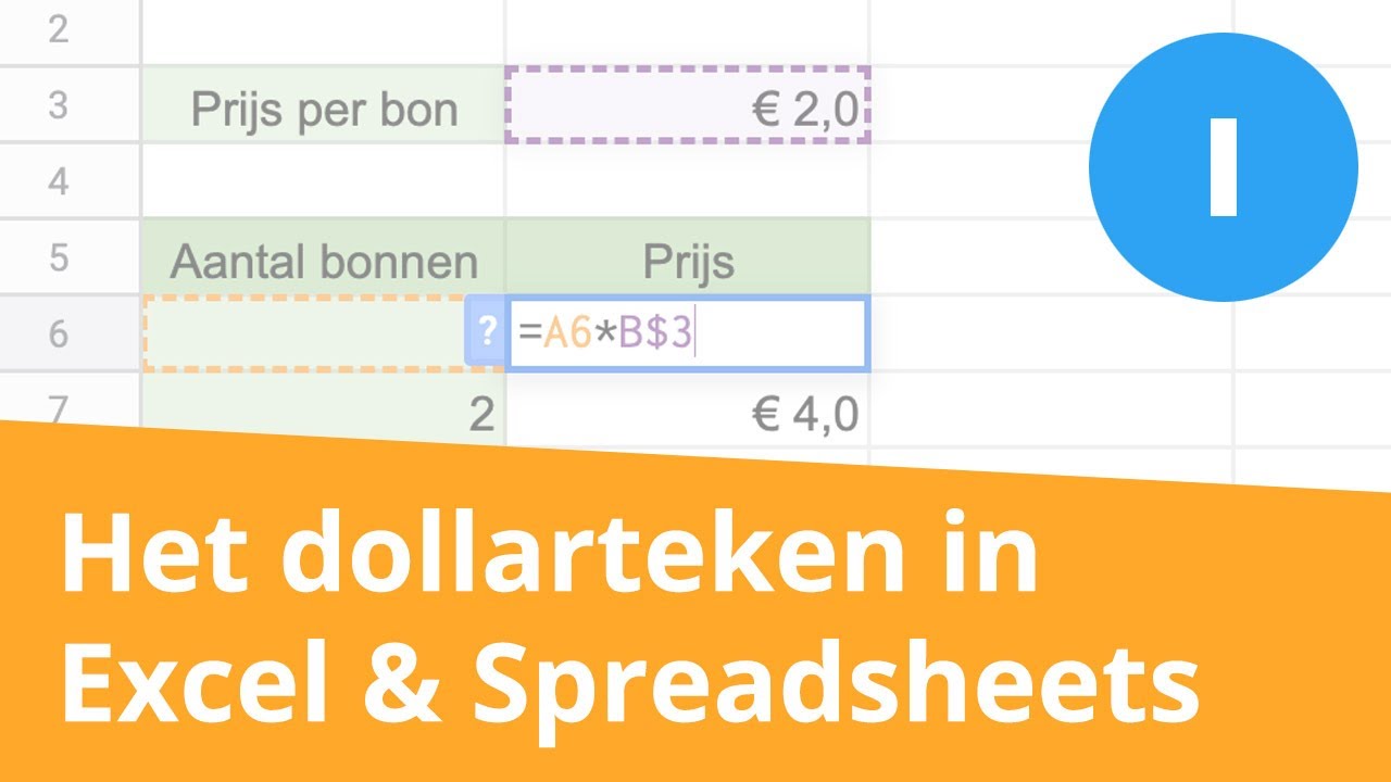
• 🔢 In more complex examples, the dollar sign is used to fix certain parts of a formula while allowing others to adjust, such as when calculating revenue based on price and quantity.
• 💡 The IF statement is combined with dollar signs to create conditional formulas, such as awarding a bonus based on revenue thresholds.
• 📋 The INDEX MATCH function is introduced in a complex scenario to dynamically reference data based on both row and column criteria, with dollar signs used to control which parts of the formula adjust.
• 🎓 The video concludes with a recommendation to watch a more in-depth video on INDEX MATCH or to take an Excel course for further learning.

Q & A

What is the main topic of the video?

The main topic of the video is understanding how to correctly use dollar signs in Excel for cell referencing.

Why is knowing where to put the dollar sign in Excel important?

Knowing where to put the dollar sign in Excel is important because it determines whether a cell reference is fixed (absolute) or dynamic (relative), which affects how formulas are copied and filled across cells.

What is the purpose of the five examples provided in the video?

The purpose of the five examples is to demonstrate the correct use of dollar signs in different scenarios, ranging from simple to complex, to help viewers understand how to lock either the column, row, or both in cell references.

What is the first example in the video about?

The first example is about calculating tax amounts for a table of products, illustrating how to lock the cell reference for the sales tax percentage while allowing the price to change as the formula is copied down.

How does the video demonstrate fixing the reference for the sales tax percentage in the first example?

The video demonstrates fixing the reference for the sales tax percentage by using the F4 key to add a dollar sign in front of the column letter and row number, making it absolute.

What is the second level example in the video about?

The second level example is about applying different tax rates for various countries, showing how to lock the tax rate reference to the correct column while allowing it to move across rows for different products.

How can you lock a cell reference to a specific column but allow it to move across rows?

You can lock a cell reference to a specific column by adding a dollar sign in front of the column letter and leave the row number without a dollar sign, allowing it to move across rows.

What is the purpose of the CHART templates mentioned in the video?

The CHART templates are used to visualize data in various chart types, allowing users to easily modify data and have the charts update automatically, helping to decide which chart type suits their data best.

How does the video handle more complex scenarios with formulas like IF statements?

The video handles complex scenarios with IF statements by showing how to lock and unlock parts of the formula correctly using dollar signs to ensure that the logic of the formula is maintained when copied across cells.

What is the most complex example discussed in the video?

The most complex example is using the INDEX MATCH formula to calculate revenue for different years and line items, demonstrating how to lock and unlock parts of the formula to ensure it works correctly when copied across cells.

How can you lock a cell reference to a specific row but allow it to move across columns?

You can lock a cell reference to a specific row by adding a dollar sign in front of the row number and leave the column letter without a dollar sign, allowing it to move across columns.

Outlines

00:00

🔍 Understanding Dollar Signs in Excel Formulas (Level 1)

This paragraph introduces the concept of using dollar signs in Excel formulas to fix cell references. The speaker demonstrates the issue of cell references changing incorrectly when formulas are dragged, and explains how to use the F4 key or manually add dollar signs to lock the reference. The example involves calculating sales tax for products, and the focus is on locking the sales tax reference while allowing the product price reference to adjust as the formula is dragged.

05:01

🌍 Handling Multiple Tax Rates in Excel (Level 2)

This section moves to a more complex example where different tax rates are applied for multiple countries (US, Japan, Mexico). It explains how to adjust Excel formulas for cell references that need to change horizontally (across countries) while locking certain cells vertically (for products). The speaker shows how to apply partial dollar sign locking to ensure the correct movement of values in both directions, demonstrating the challenge of copying formulas across rows and columns.

10:01

💰 Multiplying Prices and Quantities with Locked References (Level 3)

Here, the script covers the task of calculating revenue by multiplying product prices by quantities. The problem arises when copying the formula across cells without locking the appropriate rows and columns. The speaker highlights the need to lock the row for the quantities and the column for the prices to prevent errors in calculations when dragging formulas. The demonstration explains using the F2 key to edit formulas and adding dollar signs for precise reference control.

🔢 Combining IF Statements with Dollar Signs (Level 4)

This section dives into using the IF function in Excel combined with locked cell references. The scenario involves calculating bonuses for revenue figures that exceed a specific threshold (50,000). The speaker explains how to use the F4 key to lock specific parts of the formula, ensuring that the bonus calculation works correctly when the formula is dragged down. The focus is on controlling the movement of references to revenue and bonus percentages.

📊 Complex Formula with INDEX and MATCH Functions (Level 5)

The final and most advanced example involves using the INDEX and MATCH functions to retrieve data from an income statement. The speaker explains how to use dollar signs to lock specific cell ranges and ensure that the formula can move correctly both horizontally (across years) and vertically (across line items like net income and gross profit). This complex formula demonstrates how to combine multiple functions with careful use of locked references to get the right data from a dynamic table.

Keywords

💡Dollar Sign

The dollar sign in Excel is used to create absolute references in formulas. It is crucial for ensuring that certain parts of a cell reference do not change when the formula is copied to other cells. In the video, the dollar sign is explained as a tool to 'lock' either the column, row, or both in a cell reference, which is essential for accurate calculations when dealing with dynamic data. For instance, the script mentions locking the 'B3' cell to ensure the price remains constant while the tax percentage changes.

💡Cell Reference

A cell reference in Excel is the address of a cell, such as 'B3', used to identify its location in a worksheet. The video script discusses how to manipulate cell references using the dollar sign to ensure formulas perform as expected when copied or filled across different cells. For example, the script explains how to lock the reference to 'B3' to keep the price static while the tax rate varies.

💡Formula

A formula in Excel is an equation that performs calculations on values in cells. The script provides examples of formulas used to calculate tax amounts, revenue, and bonuses, illustrating how to construct and adjust them for dynamic referencing. The video emphasizes the importance of formulas in Excel for automating calculations and making data analysis more efficient.

💡Absolute Reference

An absolute reference in Excel uses the dollar sign to lock either the row, column, or both in a cell reference, ensuring it does not change when the formula is copied. The video script uses examples such as locking the 'B3' cell to demonstrate how absolute referencing can maintain consistency in calculations across different cells.

💡F4 Key

The F4 key in Excel is used to toggle between relative and absolute cell references. The video script instructs viewers on using the F4 key to lock cell references, which is crucial for creating formulas that function correctly when copied to other cells. This is demonstrated in the context of calculating tax amounts and handling different tax rates for various countries.

💡Drag and Drop

In the context of the video, drag and drop refers to the action of copying a formula down or across cells in Excel. This is a common method for applying the same calculation to a range of cells. The script explains how to use drag and drop effectively after locking cell references with the dollar sign to ensure formulas remain accurate.

💡Sales Tax

Sales tax is a tax imposed on the sale of goods and services. The video script uses sales tax as a practical example to demonstrate how to calculate tax amounts in Excel. It shows how to create a formula that multiplies the price by the sales tax percentage and how to adjust the formula to handle different tax rates for different countries.

💡Revenue

Revenue in the video script refers to the income generated from the sale of products. It is used in a scenario where the video explains how to calculate revenue by multiplying the price by the quantity sold. The concept of revenue is central to understanding financial performance and is a key metric in business analysis.

💡IF Statement

An IF statement in Excel is a logical test that returns one value if a condition is true and another if it is false. The video script includes an example where an IF statement is used to give a bonus based on revenue. It demonstrates how to structure the IF statement within a formula to perform conditional calculations.

💡INDEX MATCH

The INDEX MATCH function in Excel is used to look up values in a table or range. The video script provides a complex example of using INDEX MATCH to find revenue for specific years and line items. It shows how to construct the function to reference data accurately without confusion, which is essential for financial reporting and analysis.

Highlights

Understanding the confusion around the placement of dollar signs in Excel formulas.

Level 1 example introduces the concept of locking a cell reference with the F4 key.

Explanation of how to fix the formula when dragging it down in Level 1 by locking the sales tax percentage with the dollar sign.

Introduction to more complex scenarios with different tax rates for multiple countries in Level 2.

Clarification on when to lock the row or column using the dollar sign for sideways and vertical movement.

Demonstrating the process of applying the formula to different columns and rows while maintaining proper references.

Detailed explanation of how to selectively lock rows and columns to prevent errors when copying formulas across different areas.

Highlighting the use of more advanced formulas like IF statements combined with dollar signs in Level 4.

Locking row references while keeping the column dynamic for a more complex bonus calculation.

Introduction to index-match formulas in Level 5 for retrieving data from a larger table based on multiple criteria.

Explanation of how to properly lock ranges in index-match formulas to ensure correct results when dragging the formula across rows and columns.

Visualization of proper cell referencing and locking techniques through more complex examples.

Emphasizing the importance of understanding when to lock only the column, row, or both in formulas.

Using the F4 key to toggle between locking the row, column, or both in Excel, demonstrated multiple times across examples.

Encouragement to practice these skills with downloadable exercises provided in the video description.

Transcripts

one of the most confusing things in

Excel is knowing where to put the dollar

sign is it before the cell column letter

or is it before the cell row number or

is it in both this took me months to

learn correctly but by the end of this

video it should be crystal clear and for

this we'll go over five examples from

easy to hard so let's get into

[Music]

it first up in level one we have this

example table over here which has the

price of certain products alongside the

sales tax and we want to calculate the

tax amounts now if you want to follow

along with this one and all the other

exercises that we have download the free

Excel file in the video description all

we need to do for this calculation is

select the price and multiply that by

the sales tax percentage and hit enter

that's looking good at 1% and now we can

just drag this down but you'll notice as

we do that they all go to zero if we

double click on it which is the same

thing as pressing the F2 key you'll

notice that this is going down the sales

tax is going down where it shouldn't but

we do want the price to go down much

like it did here so we somehow need to

just fix this part so it stays locked at

this top B3 cell so we can go back to

the top one select it with the F2 key

and from here we're just going to select

the B3 area and press the F4 key if you

can't find the F4 key on your keyboard

board you can also just type the dollar

signs manually in front of the B and the

three now as I double click on this

again to drag it down you'll notice that

it stays fixed on this side but it

remains Dynamic so it keeps going down

on this other side for the blue price

that's a simple example of when the

dollar sign comes Hy but this one was

overly simplified let's go over a

slightly harder one in level two here

you'll notice that we have several

different tax rates for each country so

for the US us Japan and Mexico so we'll

get started with the US in the same way

as before where we take the price and

multiply that by the US tax percentage

but this time we'll lock it with the F4

key like we did earlier hit enter and we

can just drag this down by selecting the

corner so you can see that it's working

well even for different products you'll

notice that it's moving the right way

that said if we copy this formula with

crl c and contrl V to paste it over to

Japan let's click on that to see what's

going on here it's still at the US so

that's not correct and also with the

price it's actually moved one over to

the US tax as the price which is just

completely wrong so we really need to do

two things here one is going to be to

make this one Dynamic to the side not up

and down though just sideways on row

number three and for this one we want to

keep it fixed at column G but be able to

move up and down so let's get inside the

formula again at the very first one and

we need to make the changes here so for

G3 which is this one right here that we

can't quite see right now we want to add

a dollar sign on the column so that it

doesn't move to other columns we can do

that just by adding the dollar sign on

that g there for the number it's row

number three we do want it to move

because we want it to go across the

different products so we leave that as

is then on this other side for the B3 we

want it to move across the col s so from

b c to D that's why we'll delete the

dollar sign from there that said do we

want it on the number well we do because

we don't want it to go down to row

number four five or six where there's

actually nothing in it now we can just

hit enter and we'll copy this formula

and just drag it down and across just

shift down arrow to go to the bottom

there and shift right arrow to go to the

right and then I can just hit contrl V

now you'll notice that it should be

working correctly we can just check the

last one by double clicking on it you

can see that the price has gone down all

the way to Doritos and we're using the

Mexico tax rate which makes sense for

the Mexico column awesome now you've

seen when to add the dollar signs just

for the column just for the row as well

as for both and the next step would be

to visualize all of this and to do that

we can use charart templates like the

ones hotspot is kindly providing us

using the link in the description Bel

below you can get multiple graph

templates completely for free in the

download you'll find an Excel file with

the instructions on using the template

alongside all of the chart types you

might need to visualize your data from

here you can easily modify the data and

the charts will automatically update

these templates can have either one

column of data or multiple depending on

your needs I personally find this

template useful for deciding which chart

type suits my dat the best as it's quite

unusual to see so many different chart

types in just one template so I'd

recommend you head out to the link in

the description below to download these

completely free templates from hopspot

to level up your Excel game and thanks

to them for sponsoring this video we've

just gone over two examples of sell

referencing but to be fully confident

let's go over another slightly different

example over here it just says to find

the revenue under the scenarios and you

can see we have all the prices on one

side and all the quantities on the other

and based on that we want to multiply

each of them so it would be 10

multiplied by 250 to find the revenue

under these conditions and we want to

move this all across so if we just try

to do that now just by dragging this

down let's see what happens if I click

on this one you'll notice that it's not

moving correctly at least from this top

part and if I were to copy this across

to the side and take a look at this with

the F2 key you'll notice that it's also

not moving correctly because the

quantity should be fixed here so we need

to fix two things one is going to be

this column C and the other one is going

to be this row five so let's take a look

here we'll press the F2 key to get

inside of the formula and the first part

is going to be this number 10 that we do

want to move across so across the

different columns but we want it to stay

fixed at row five so we'll add the

dollar sign only at the row number four

five then we have the C6 which we want

it to remain at this column C so it

doesn't move to the other columns and

make everything wrong so we just need to

add the dollar sign in front of that c

we'll hit enter there crl C to copy

shift down shift right to select the

whole area and now contrl V to paste it

all to check if it's all working

correctly we can just go to the very

last one and you'll see that it's gone

all the way to 16 and the quantity all

the way to 1,000 so that's all looking

correct up till now we've been working

with fairly simple scenarios where it's

only one calculation in reality though

you'll probably mix this with a formula

like an if statement which is what we

look at in this level four over here we

have the instructions in bold and it

says that if the revenue here is greater

than 50,000 then we want to give them a

5% bonus probably of the total revenue

so over here we're going to need an F

so we'll go to equals if hit the top key

there The Logical test is that this

Revenue figure over here has to be

greater than that 50,000 which is right

here to the side that said right now if

we drag this down it's all going to get

messed up so we should try to lock this

with the F4 key you'll notice we can

either lock by column and row that's one

way to do it there's nothing wrong with

it or the other way for us to do it

would be to just lock the row so we

would only lock the five area over here

that would give us the same effect

because we don't really need to move the

bonus to other areas like left or right

now if that is the case so if the value

is true we want to multiply the revenue

itself which we can't quite see it's

just a C5 multiply it by the Bonus

percentage and again we can leave the

dollar sign in the same way as over here

so we can press the F4 ke key not once

but twice so that the dollar sign is

just on the end you'll have notice there

that as you press the F4 key the dollar

sign keeps moving to wherever you would

want it there and now comma and if the

value is false they don't get a bonus so

we'll just put nothing in there with two

quotations that's all for this one we'll

close the parenthesis and hit enter now

we can double click there to drag this

down and let's say we take a look at

this one over here you'll notice this

area is working correctly and so is this

part as it's moved down to C8 and

because this figure is greater than

50,000 we do get that bonus that's an

example of us using the F statement and

the dollar signs and now in level five

we'll go over something much much harder

and I'm not expecting everyone to get

this on the first try as it's quite

complex over here you can see that we

have an income statement down below and

on this top part we want to find out

what's the revenue in 2021 and then be

able to move that formula cross all the

way to 2023 and on different line items

as well for this we're going to need an

index match so we'll go ahead and add

that formula in first and then we'll

take a look at where to add the dollar

signs so let's get started with equals

index hit the top key there and the

array is basically all of the numbers or

the results we're interested in which is

going to be all of these over here you

can see I've highlighted them comma and

now we want to add the first match so

there's two matches here one is going to

be the row match and the other the

column match from the row perspective we

have all of these different rows here so

the first match that we want the local

value is we want to find out the revenue

comma where can we find the revenue that

would basically be the array well we can

find it in this bottom area over here

comma and we want this to be an exact

much we'll put a zero for that close up

parenthesis comma and we'll now go over

a second match Lo at Value is we're

looking for the year comma and we're

looking for the year among all of these

years over here to the side hit the

comma and we want an exact match close

the parenthesis and now we need to close

it again but this time for the index

side close that and just hit enter so we

have

229,000 in Revenue which if we take a

look that looks about right it's this

figure right here that said if I move

this down let's say I move it just one

down let's take a look at this value

here this one's clearly off because all

of this bottom areas move down by one

same thing goes with this top part the

only part that's correct right now is

the gross profit so that's really not

looking good that's because we haven't

locked the sales correctly with the

dollar signs so let's take a look up

over here the index this whole area with

the numbers really doesn't have to move

at all so we'll put the dollar signs all

across but selecting it and pressing the

F4 key once now for the match itself the

revenue here you can see the B4 we want

it to move down but not across so for

this we're going to lock it at the

column that way it can't move across the

different columns secondly for all of

the values that we have here on the

bottom we're not going to have to move

them at all so to make things simple we

can also just hit the F4 key ones to

lock them all across and finally for

this last part which really has to do

with that year there we want it to move

sideways but not up and down so we just

want the dollar sign on the three there

and then for this second part it's not

going to move at all so we can just

press the F4 key all across it now hit

enter that answer shouldn't change but

now as we drag this down and across so

crl C to copy shift down arrow shift

right arrow and contrl + V to paste now

let's take a look at at net income 2023

this has moved correctly to 2023 same

thing with net income and if we take a

look at the figure 2023 net income is

53,000 so that's all looking good if

this index match formula was a bit

confusing for you don't worry check out

this video over here where I go over it

in a lot more depth or by taking our

Excel course over here hit the like and

that subscribe and I'll catch you in the

next one