Numerical Integration With Trapezoidal and Simpson's Rule
Summary
TLDRThis educational video script delves into numerical integration, a method for approximating definite integrals that are difficult to solve analytically. It introduces two primary techniques: the trapezoidal rule and Simpson's rule. The trapezoidal rule is explained through a step-by-step process, emphasizing the calculation of ΔX, the use of function evaluations at incremental points, and the summation formula. The script then contrasts this with Simpson's rule, which alternates between multiplying function evaluations by four and two, requiring an even number of intervals for accuracy. Practical examples, including calculating integrals of 1/x from 1 to 2 and 1/√(x+1) from 0 to 2, demonstrate the application of these methods, showing how they can closely approximate true integral values, even when exact solutions are unknown.
Takeaways
- 🔢 Numerical integration is a method used to approximate definite integrals that cannot be solved using traditional calculus techniques.
- 📐 The Trapezoidal Rule is one such method, which approximates the area under a curve by dividing it into trapezoids rather than rectangles.
- ∆x The Trapezoidal Rule formula involves calculating the sum of function values at intervals (∆x) multiplied by their respective coefficients and then taking the average.
- 📉 The Simpsons Rule is another numerical integration technique, which uses a more complex formula involving the sum of function values at intervals multiplied by coefficients that alternate between 4 and 2.
- 🔁 Both the Trapezoidal and Simpsons Rules require the number of intervals (N) to be specified, with the Simpsons Rule needing an even number of intervals for accuracy.
- 📋 The script provides a step-by-step example of how to apply the Trapezoidal Rule to approximate the integral of 1/x from 1 to 2 using 10 intervals.
- 📘 The script also demonstrates the application of the Simpsons Rule using the function 1/√(x+1) from 0 to 2 with 7 intervals, emphasizing the need for even intervals.
- 🔍 The accuracy of numerical integration methods improves as the number of intervals increases, leading to a better approximation of the actual integral.
- 📊 The script compares the results of the numerical integration methods with the actual integrals when possible, showcasing the closeness of the approximations.
- 💡 The script serves as a tutorial for students who may not have covered certain integrals in their calculus courses, providing an alternative approach to finding area under curves.
Q & A
What is numerical integration?
-Numerical integration is a method used to approximate definite integrals that cannot be solved analytically, providing a way to estimate the area under a curve when an exact formula is not known or available.
What are the two main methods of numerical integration discussed in the script?
-The two main methods of numerical integration discussed in the script are the trapezoidal rule and Simpson's rule.
How does the trapezoidal rule work?
-The trapezoidal rule works by approximating the area under a curve by dividing the area into trapezoids rather than rectangles. It sums the areas of these trapezoids to approximate the definite integral.
What is the formula for the trapezoidal rule?
-The formula for the trapezoidal rule is given by \(\Delta x \frac{f(x_0) + 2f(x_1) + 2f(x_2) + \ldots + 2f(x_{n-1}) + f(x_n)}{2}\), where \(\Delta x\) is the width of each trapezoid, and \(f(x_i)\) represents the function evaluated at the points \(x_i\).
What is the significance of the term 'Delta X' in the context of numerical integration?
-In numerical integration, 'Delta X' (\(\Delta x\)) represents the width of the subintervals into which the area under the curve is divided to approximate the integral using either the trapezoidal rule or Simpson's rule.
Why is the number of terms (N) important in numerical integration?
-The number of terms (N) is important because it determines the accuracy of the approximation. A larger N results in more subintervals, which generally leads to a better approximation of the integral.
How does Simpson's rule differ from the trapezoidal rule?
-Simpson's rule differs from the trapezoidal rule in that it approximates the area under a curve using parabolic segments instead of trapezoids. It uses a different weighting for the function evaluations, with the first and last terms having a coefficient of 1, the middle terms having a coefficient of 4, and every other term having a coefficient of 2.
What is the formula for Simpson's rule?
-The formula for Simpson's rule is given by \(\frac{\Delta x}{3} [f(x_0) + 4f(x_1) + 2f(x_2) + 4f(x_3) + 2f(x_4) + \ldots + 2f(x_{n-2}) + 4f(x_{n-1}) + f(x_n)]\), where n must be an even number.
Why does Simpson's rule require an even number of terms (N)?
-Simpson's rule requires an even number of terms because it relies on the parabolic shape that is formed between every two points, and this requires pairs of intervals to create the parabolic segments for the approximation.
How can one improve the accuracy of numerical integration using the trapezoidal or Simpson's rule?
-The accuracy of numerical integration can be improved by increasing the number of terms (N), which results in smaller subintervals and a more detailed approximation of the curve's shape.
What is the practical application of numerical integration?
-Numerical integration is used in various fields where exact integration formulas are not available or practical, such as in physics for calculating work done, in engineering for stress analysis, and in computer graphics for rendering.
Outlines

This section is available to paid users only. Please upgrade to access this part.
Upgrade NowMindmap

This section is available to paid users only. Please upgrade to access this part.
Upgrade NowKeywords

This section is available to paid users only. Please upgrade to access this part.
Upgrade NowHighlights

This section is available to paid users only. Please upgrade to access this part.
Upgrade NowTranscripts

This section is available to paid users only. Please upgrade to access this part.
Upgrade NowBrowse More Related Video

LENGKAP Integral tak tentu, integral tertentu, integral subtitusi dan integral parsial
Integration By Parts
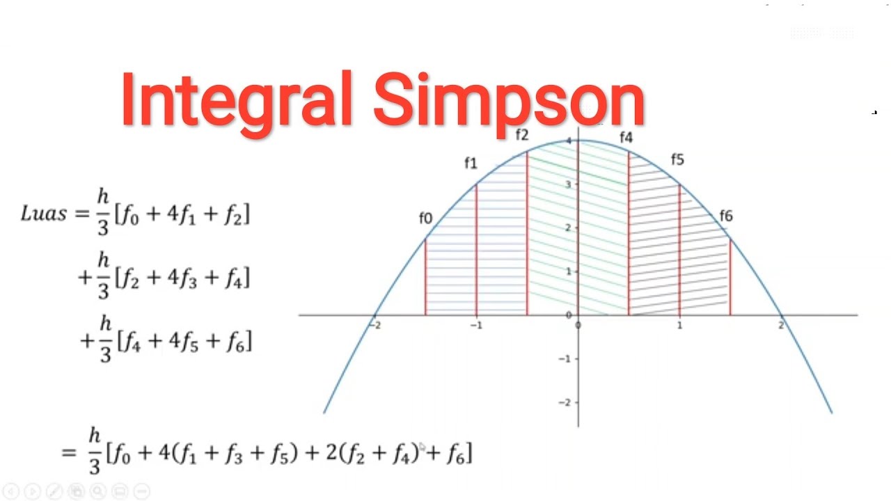
Integral Numerik dengan metode Simpson serta kode Pythonnya.

Integrales definidas | Ejemplo 1
¿Qué es la INTEGRAL? | SIGNIFICADO de la integral definida (Lo que no te enseñan sobre la integral)

#06 Konsep Dasar Integral dalam Matematika untuk Fisika Bagian #1
5.0 / 5 (0 votes)