Top 7 Algorithms for Coding Interviews Explained SIMPLY
Summary
TLDRThis comprehensive video script delves into the seven most crucial algorithms for coding interviews: binary search, depth-first search, breadth-first search, insertion sort, merge sort, quick sort, and greedy algorithms. It meticulously explains each algorithm's mechanism, real-life applications, time complexity, and when to utilize them effectively. Through insightful visualizations and relatable examples, the script offers a deep understanding of these fundamental algorithms, empowering viewers to excel in coding interviews and strengthen their problem-solving abilities.
Takeaways
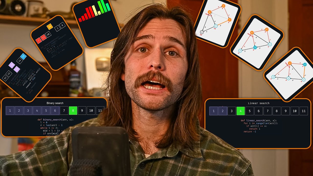
- 😃 Binary search is an efficient search algorithm for sorted lists, with a time complexity of O(log n).
- 🤖 Depth-first search (DFS) and breadth-first search (BFS) are crucial algorithms for traversing trees and graphs, commonly used in coding interviews.
- 🧮 Insertion sort is a simple sorting algorithm with a time complexity of O(n) for best case and O(n^2) for worst case, suitable for small or mostly sorted lists.
- 📈 Merge sort is a divide-and-conquer sorting algorithm with a time complexity of O(n log n), efficient for larger, unsorted lists.
- 🔄 Quick sort is a divide-and-conquer sorting algorithm with a time complexity of O(n log n) for the average case, but can degrade to O(n^2) for the worst case. It is generally faster than merge sort on average but harder to implement correctly.
- 💰 Greedy algorithms make the locally optimal choice at each step, without considering the global optimum. They are useful when finding the exact optimal solution is computationally infeasible.
- 🧭 The traveling salesman problem is a classic example where greedy algorithms can provide a reasonably good approximation when finding the exact optimal solution is impractical due to the exponential growth of possible routes.
- 🔑 Understanding time complexity is crucial for evaluating and comparing the efficiency of different algorithms.
- 📚 Familiarity with basic data structures, such as arrays, trees, and graphs, is essential for understanding and implementing these algorithms effectively.
- 🚀 Mastering these algorithms is essential for coding interviews, as they are among the most commonly asked questions, particularly for data structures and algorithms.
Q & A
What are the three search algorithms discussed in the script?
-The three search algorithms discussed are binary search, depth-first search (DFS), and breadth-first search (BFS).
What is the time complexity of the binary search algorithm?
-The time complexity of the binary search algorithm is O(log n).
What is the difference between depth-first search (DFS) and breadth-first search (BFS)?
-DFS explores as far as possible along each branch before backtracking, while BFS explores all the nodes at the current level before moving on to the next level.
What is the time complexity of DFS and BFS?
-Both DFS and BFS have a time complexity of O(V + E), where V is the number of vertices (nodes) and E is the number of edges (connections).
What are the three sorting algorithms discussed in the script?
-The three sorting algorithms discussed are insertion sort, merge sort, and quick sort.
What is the best-case and worst-case time complexity of insertion sort?
-The best-case time complexity of insertion sort is O(n), and the worst-case time complexity is O(n^2).
What is the time complexity of merge sort?
-The time complexity of merge sort is O(n log n) for both the best and worst cases.
What is the best-case and worst-case time complexity of quick sort?
-The best-case time complexity of quick sort is O(n log n), while the worst-case time complexity is O(n^2).
What is a greedy algorithm, and when is it used?
-A greedy algorithm is an algorithm that makes the best possible choice at every local decision point. It is used when finding the optimal solution might not be possible, and we want to find a relatively accurate solution.
Can you provide an example of a problem where a greedy algorithm might be useful?
-The traveling salesman problem, where the goal is to find the shortest possible route that visits each city once and returns to the origin city, is a good example of a problem where a greedy algorithm might be useful when the number of cities becomes too large to calculate the optimal solution.
Outlines

This section is available to paid users only. Please upgrade to access this part.
Upgrade NowMindmap

This section is available to paid users only. Please upgrade to access this part.
Upgrade NowKeywords

This section is available to paid users only. Please upgrade to access this part.
Upgrade NowHighlights

This section is available to paid users only. Please upgrade to access this part.
Upgrade NowTranscripts

This section is available to paid users only. Please upgrade to access this part.
Upgrade NowBrowse More Related Video
3 Types of Algorithms Every Programmer Needs to Know

Searching Algoritms - Linear and Binary Search

Learn Searching and Sorting Algorithm in Data Structure With Sample Interview Question

Algorithms Explained for Beginners - How I Wish I Was Taught
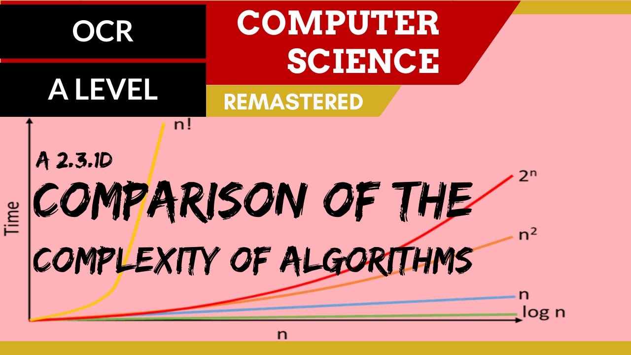
161. OCR A Level (H446) SLR26 - 2.3 Comparison of the complexity of algorithms

TIK-Pencarian dan Pengurutan
5.0 / 5 (0 votes)