Cara VLOOKUP Data ke Kiri dengan Rumus Index Match | Tutorial Excel Pemula - ignasiusryan
Summary
TLDRIn this tutorial, the presenter introduces viewers to an alternative to VLOOKUP in Excel—using the INDEX and MATCH functions. The video demonstrates how INDEX and MATCH allow you to search for data even when the lookup column is not the first column, overcoming VLOOKUP's limitation. By explaining the formula and applying it to a real-world example with customer data, the tutorial guides users step by step on how to automate data retrieval efficiently. Viewers are encouraged to practice using these formulas for larger datasets and are invited to engage with the content by liking, commenting, and subscribing.
Takeaways
- 😀 VLOOKUP has a limitation: it requires the reference column to be the leftmost column in the data.
- 😀 INDEX MATCH is a powerful alternative to VLOOKUP that allows you to perform lookups even if the reference column isn't the first column.
- 😀 The INDEX function retrieves data from a specified row and column in a reference table.
- 😀 The MATCH function helps to find the row number for a specific reference in a given range, automating part of the lookup process.
- 😀 Combining INDEX and MATCH allows for dynamic lookups, even when the reference data is in the middle or far-right of the table.
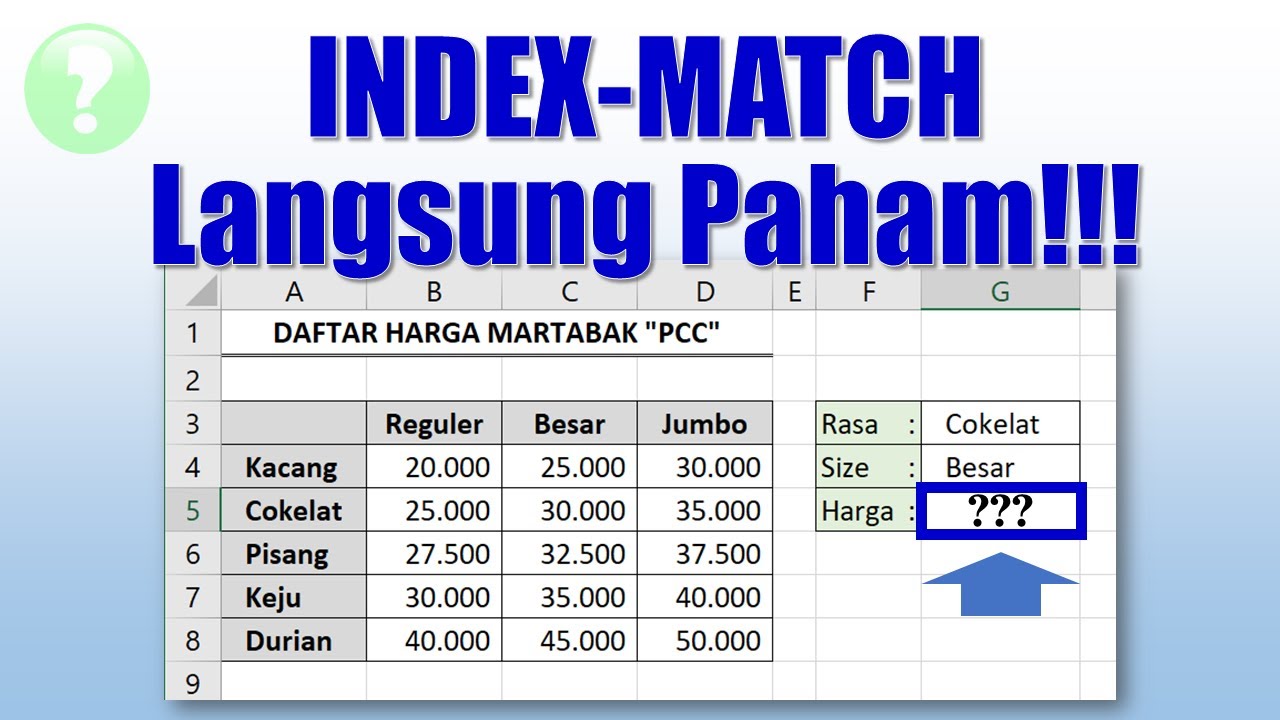
- 😀 The formula structure for INDEX MATCH is: =INDEX([Table], MATCH([Lookup Value], [Lookup Column], 0), [Column Number]).
- 😀 To avoid errors when copying the formula, use absolute references (F4) to lock the reference range.
- 😀 With INDEX MATCH, you can retrieve data from any column, regardless of its position in the table.
- 😀 When you need to look up multiple data points, you can drag the formula down to automatically populate other rows.
- 😀 For complex tables with multiple data points, INDEX MATCH offers more flexibility and precision than VLOOKUP.
- 😀 INDEX MATCH can be used for both simple and complex lookups, making it a versatile tool for Excel users.
Q & A
What is the main focus of the video script?
-The video focuses on explaining how to use the INDEX and MATCH functions in Excel to search for data when the reference cell is not in the first column, unlike the VLOOKUP function which requires the reference to be in the leftmost column.
Why can't VLOOKUP be used when the reference column is not the first column?
-VLOOKUP requires the reference column to be the first column in the table range. This limitation prevents it from being used when the reference data is in a column that is not the leftmost one.
What is the alternative to using VLOOKUP for non-leftmost reference columns?
-The alternative is using the combination of the INDEX and MATCH functions. This method allows searching for data in columns that are not the leftmost, offering more flexibility than VLOOKUP.
How does the INDEX function work in this tutorial?
-The INDEX function retrieves data from a specified table by selecting a row and column. In the video, it is used to extract the customer name by providing the reference table, row number, and column number.
What role does the MATCH function play in this approach?
-The MATCH function is used within the INDEX function to automatically find the row number where the reference value (e.g., order number) is located. This eliminates the need for manual row number entry.
What is the significance of using the $ symbol in the formula?
-The $ symbol is used in the formula to lock the cell reference when copying the formula down the column. This prevents the reference from changing as the formula is dragged to other cells.
What is the structure of the INDEX-MATCH formula used in this tutorial?
-The structure is: =INDEX(reference_table, MATCH(reference_value, lookup_column, 0), column_number). The INDEX function retrieves the data from the reference table, and MATCH finds the row corresponding to the reference value.
How does the MATCH function ensure the search is exact?
-The MATCH function uses a '0' argument, which specifies that the search should be exact. This ensures the function finds the exact match for the reference value in the lookup column.
Why is it necessary to use the MATCH function with INDEX in this case?
-The MATCH function is necessary because it automates the process of finding the row number for a specific reference value. Without it, the user would have to manually input the row numbers, which is inefficient for large datasets.
What example is used in the tutorial to demonstrate the INDEX-MATCH technique?
-The tutorial uses a table with order numbers in the last column, customer names in the first column, and customer locations in the third column. The example demonstrates how to extract customer names and locations based on the order number, even when the order number is not in the first column.
Outlines

このセクションは有料ユーザー限定です。 アクセスするには、アップグレードをお願いします。
今すぐアップグレードMindmap

このセクションは有料ユーザー限定です。 アクセスするには、アップグレードをお願いします。
今すぐアップグレードKeywords

このセクションは有料ユーザー限定です。 アクセスするには、アップグレードをお願いします。
今すぐアップグレードHighlights

このセクションは有料ユーザー限定です。 アクセスするには、アップグレードをお願いします。
今すぐアップグレードTranscripts

このセクションは有料ユーザー限定です。 アクセスするには、アップグレードをお願いします。
今すぐアップグレード関連動画をさらに表示

Rumus VLOOKUP, HLOOKUP dan XLOOKUP di Excel

VLOOKUP in Excel | Step-by-Step Tutorial for Beginners
Cara Menggunakan Rumus Index Match di Excel
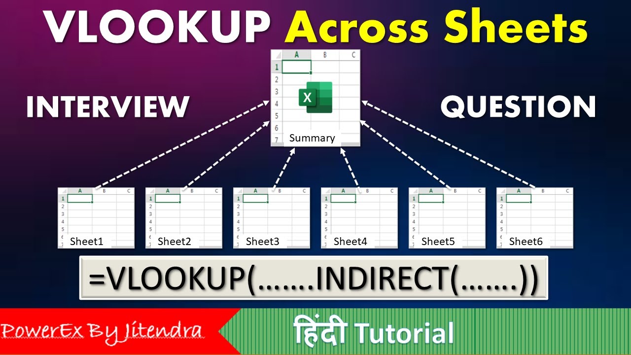
VLOOKUP Across Sheets | VLOOKUP + INDIRECT | VLOOKUP MATCH | MIS Interview Question

Cara Menggunakan Fungsi MATCH, INDEX & CHOOSE dalam Ms Excel | Informatika Kelas 8 Bab Analisis Data

Cara Menggunakan Rumus Index Match
5.0 / 5 (0 votes)
