Altair Compose: Signal Processing - Power Spectral Density

Summary

This lecture introduces power spectral density (PSD) and its computation using the Discrete Fourier Transform (DFT) and the Welch method, which offers a robust way to estimate PSD in noisy signals. The lecture explains how PSD represents the distribution of signal power across frequencies and provides formulas to calculate both single-sided and double-sided PSDs. It also covers signal processing challenges like noise and frequency resolution, and demonstrates how the Welch method mitigates these issues through segmentation and overlapping. Finally, it shows practical PSD calculation using Compose, emphasizing key advantages and trade-offs.

Takeaways

• 📊 The lecture introduces Power Spectral Density (PSD), a method to represent the power of a signal distributed over a frequency spectrum.
• 📐 PSD is calculated by dividing the spectral power by the frequency range, often using the Discrete Fourier Transform (DFT) or Fast Fourier Transform (FFT).
• 🎛️ The difference between double-sided and single-sided PSDs is explained, with single-sided PSD requiring a folding process of the double-sided PSD.
• 💡 The Welsh method is introduced as a more robust algorithm for estimating PSD, useful for handling noisy or non-deterministic signals.
• 📈 The Welsh method divides a signal into overlapping segments, applies a window function, computes FFTs, and averages the PSDs to provide a more accurate representation.
• 🔄 Overlapping segments in the Welsh method ensure no loss of critical information that might occur at the edges of windows in the signal.
• 🧮 The lecture emphasizes that PSD is a density measurement, meaning it is normalized by frequency resolution, which is crucial for interpreting the results.
• ⚖️ It highlights the trade-off in using the Welsh method: while it reduces noise, it also lowers frequency resolution.
• 🔧 The practical implementation of PSD computation is shown using the Compose tool, leveraging built-in functions such as 'P Welch' to simplify the process.
• 🎮 The provided app allows users to experiment with different parameters (e.g., window type, overlap, window length) to visualize their effects on the PSD and signal.

Q & A

What is Power Spectral Density (PSD)?

Power Spectral Density (PSD) represents the power of a signal distributed over its spectrum of frequencies. It describes how the power of a signal varies with frequency and is defined as power per unit frequency.

How is the Power Spectral Density (PSD) computed using the Discrete Fourier Transform (DFT)?

The PSD is computed by squaring the Discrete Fourier Transform (DFT) coefficients and then dividing by the number of coefficients to get the spectral power. The spectral power is then divided by the frequency range, which for a double-sided DFT, is the sampling frequency.

What is the difference between single-sided and double-sided PSD?

Double-sided PSD considers both positive and negative frequencies, while single-sided PSD focuses only on positive frequencies. The single-sided PSD is computed by folding the double-sided PSD and doubling the values, except for the mean and Nyquist frequency components.

What is the Parseval’s Theorem and how is it related to PSD?

Parseval’s Theorem states that the total energy of a signal can be computed equivalently in time or frequency domains. In the context of PSD, it implies that the sum of power in the time domain can be represented as the sum of spectral power in the frequency domain.

What are the advantages of the Welch method for PSD estimation?

The Welch method improves PSD estimation by averaging over multiple segments of a signal, which reduces noise and provides a better representation of the signal’s power spectrum. It also helps in estimating the PSD for non-deterministic processes.

Why is it important to use windowing in the Welch method?

Windowing helps reduce spectral leakage by minimizing the discontinuities at the edges of each segment. This allows for a more accurate estimation of the PSD, especially when dealing with overlapping segments in the Welch method.

How does the overlap of segments affect the Welch method?

Overlapping segments in the Welch method increases the usage of signal data, especially at the edges where the window function reduces the signal's impact. This leads to a more efficient use of the signal and provides a better estimate of the PSD.

What are the effects of noise on PSD computation?

Noise affects the accuracy of PSD computation by introducing additional power across the frequency spectrum. Averaging multiple segments in the Welch method helps reduce the impact of noise and provides a more robust estimate of the true PSD.

How does the length of the FFT affect the PSD resolution?

The length of the FFT determines the frequency resolution of the PSD. A longer FFT provides finer frequency resolution but may require zero-padding if the signal length is shorter. A shorter FFT reduces resolution but may be faster to compute.

What are some common applications of PSD analysis?

PSD analysis is used in signal processing to identify the frequency components of a signal, detect noise levels, and analyze random processes. It is commonly applied in fields such as telecommunications, audio processing, and vibration analysis.

Outlines

00:00

📊 Introduction to Power Spectral Density (PSD)

The video introduces Power Spectral Density (PSD), explaining that the lecture is divided into two parts. The first part covers the definition of PSD and how to calculate it using the Discrete Fourier Transform (DFT). The second part explores the Welsh method, a more robust way to compute PSD. The speaker defines PSD by breaking down its components: 'Power' refers to the signal's power, 'Spectral' refers to its distribution over frequencies, and 'Density' refers to power per unit frequency. A mathematical approach is provided to compute PSD using DFT coefficients, which are derived from the FFT algorithm. The explanation covers double-sided and single-sided PSD, and practical exercises in COMPOSE to illustrate the calculation.

05:02

📉 Why We Need the Welsh Method for PSD

This section discusses the limitations of the basic PSD computation in real-world scenarios. The speaker points out that signals are often noisy, and that PSD is typically used to analyze non-deterministic processes. To get a reliable estimate of PSD despite noise and randomness, averaging techniques like the Welsh method are useful. The Welsh method involves splitting the signal into segments, applying a window function, computing the FFT, and averaging the resulting PSDs. The key improvement in the Welsh method is using overlapping segments to avoid missing important information in the edges of the signal, thereby increasing efficiency and accuracy.

10:03

⚙️ Implementing the Welsh Method in COMPOSE

The third paragraph walks through the practical implementation of the Welsh method using the COMPOSE software. The Welsh function (pwelch) is introduced, with its various input parameters such as signal, window type, overlap, FFT length, and sampling frequency. A detailed explanation is provided on how to set the window length, define overlap (set at 50%), and adjust the FFT length. The paragraph also highlights how the Welsh method normalizes the signal, and that changing input arguments (e.g., window type or overlap) can influence the resulting PSD.

15:06

🖥️ Visualizing PSD and the Impact of Overlap

This paragraph discusses an interactive app for visualizing the PSD of a signal, showing how different parameters affect the results. The app allows users to adjust signal components (e.g., amplitudes, frequencies) and analyze how splitting, windowing, and overlapping impact the PSD. It illustrates how using an overlap of 50% makes short-duration signals, which would otherwise be lost, more visible in the PSD. The section concludes by emphasizing the importance of choosing the right overlap and window type for an accurate PSD representation.

Keywords

💡Power Spectral Density (PSD)

Power Spectral Density (PSD) represents how the power of a signal is distributed across different frequencies. In the video, PSD is the main focus, introduced as a method to visualize the power of a signal in relation to its frequency components. It is derived from the Discrete Fourier Transform (DFT) and is crucial for understanding signal behavior in the frequency domain.

💡Discrete Fourier Transform (DFT)

The Discrete Fourier Transform (DFT) converts a signal from its time domain representation to a frequency domain representation. The video explains how DFT helps in computing the power spectral density of a signal by providing the frequency components. The Fast Fourier Transform (FFT), a common algorithm for computing DFT, is used in examples throughout the lecture.

💡Welch Method

The Welch Method is a more robust approach for estimating the power spectral density of a signal, especially in the presence of noise or for non-deterministic signals. In the video, it is explained as a technique that averages the PSD over several segments of the signal, enhancing the accuracy of the estimation. The method also involves overlapping segments to preserve data at the edges of the windows.

💡Frequency Resolution

Frequency resolution refers to the ability to distinguish between different frequency components in a signal. The video highlights how frequency resolution decreases when a signal is split into multiple segments for the Welch Method, leading to trade-offs between signal length and resolution. This concept is key in understanding the limitations and advantages of PSD estimation techniques.

💡Windowing Function

A windowing function is applied to each segment of a signal in the Welch Method to reduce spectral leakage. The video explains how different windows (e.g., rectangular, Hanning) affect the resulting PSD by minimizing distortions at the edges of the signal segments. Choosing the right window is crucial for accurate PSD estimation.

💡Leakage

Leakage refers to the spreading of signal energy across multiple frequency bins, which occurs when the frequency components do not align perfectly with the FFT bins. In the video, this phenomenon is described in the context of PSD estimation, particularly when non-ideal windows are used or when frequency resolution is too low. The Welch Method helps reduce leakage by overlapping windows.

💡Sampling Frequency

The sampling frequency is the rate at which a continuous signal is sampled to convert it into a discrete form. The video discusses how the sampling frequency affects the computation of the PSD, as it determines the range of frequencies that can be represented. The formula for PSD involves dividing by the sampling frequency to normalize the spectral power.

💡FFT Algorithm

The Fast Fourier Transform (FFT) algorithm is an efficient way to compute the Discrete Fourier Transform (DFT). In the video, FFT is used to calculate the frequency components of signals, which are then used to derive the power spectral density. The efficiency of FFT is crucial for handling large datasets in signal processing applications.

💡Single-Sided Power Spectral Density

The single-sided power spectral density is obtained by folding the double-sided PSD, focusing only on the positive frequencies. The video demonstrates how to calculate it from the FFT and emphasizes its utility in cases where only positive frequency components are of interest, such as in real-valued signals.

💡Averaging

Averaging is the process of combining multiple estimates to reduce noise and obtain a more reliable PSD estimate. In the video, averaging is introduced as a key part of the Welch Method, where PSDs from different segments of the signal are averaged to produce a final estimate. This technique is essential when dealing with noisy or random signals.

Highlights

Introduction to power spectral density (PSD) and its importance in signal processing.

Explanation of the power spectral density as the power of a signal distributed over the spectrum of frequencies.

Detailed steps to compute the power spectral density using the Discrete Fourier Transform (DFT) and the Fast Fourier Transform (FFT).

Introduction of the Welch method, a more robust algorithm for calculating PSD, particularly when dealing with noisy signals or random processes.

Use of overlapping segments and window functions to improve PSD estimation and reduce leakage in the Welch method.

Explanation of single-sided and double-sided power spectral density and how to compute each using different formulas.

Hands-on approach to implementing PSD computation with the FFT algorithm and practical plotting of results.

Introduction to averaging multiple PSDs to get a more representative estimate of noisy or random signals.

Practical example of dividing a signal into overlapping segments and applying the FFT to each for more accurate PSD estimation.

Step-by-step process of implementing the Welch method in Compose, including code examples.

Introduction of random noise into the signal to simulate real-world conditions and demonstrate how noise affects PSD estimation.

Visualization and comparison of PSD results between regular FFT-based computation and the Welch method to highlight differences in frequency resolution and accuracy.

Explanation of how signal length and segment splitting affect the frequency resolution and power estimates in PSD calculations.

Exploration of different window types (e.g., rectangular, Hanning) and how they impact the accuracy of PSD in terms of reducing leakage.

Interactive app for experimenting with different PSD parameters, including window type, window length, overlap, and noise, to better understand the Welch method.

Transcripts

Hello everybody welcome back to the

signal processing playlist the main

topic of this lecture is power spectral

density

we are going to divide the lecture in

two parts in the first part we introduce

the power spectral density and we will

get a formula to compute it from the

Discrete Fourier transform of our signal

in the second part is that we will talk

about the Welsh method which is a more

robust algorithm to compute the power

Spectrum density

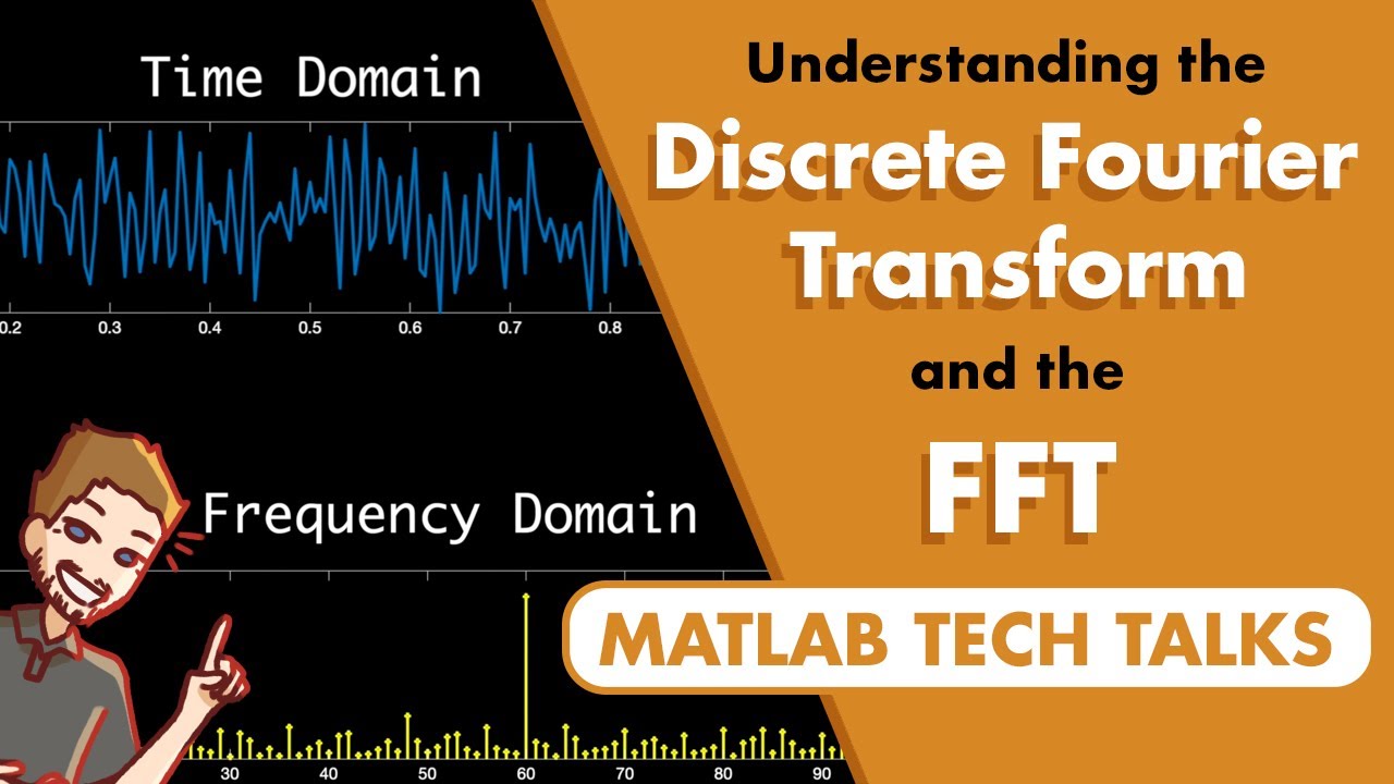
in order to better follow I understand

this lecture it's helpful that you are

familiar with Concepts such as the

description transfer and the winery

technique

now we are ready to start

the first question we have to answer is

what is power spectral density

we can get its definition by its name

so the first word is power

which means that we are representing the

power of our signal

the second war is spectral

in fact the power of the signal is

represented as a distribution over the

spectrum of frequencies

the third word is density

because this power distribution is

indeed a density

when we talk about density we are

usually thinking at mass per unit volume

these times that we are referring to

power per unit frequency

so if we think at the script for a

transform as a change of basis now with

the power spectral density we are

enriching our analysis with physical

meaning which is the power of our signal

distributed in each frequency band

and the next question is how do we

compute it

in order to get it we can leverage the

parts of a theorem

the interpretation of this theorem is

that the total energy of a signal can be

computed equivalently by

or semi Power per sample across time or

summing the spectral power across

frequency

and for the script and signals it can be

translated in mathematical language

through this formula

where the capital x stands for the

coefficient of the Discrete Fourier

transform

which more practically is what we get

from the fft algorithm

we want to get the power spectral

density so what we have to do is to

divide the spectral Power by the

frequency range we are spanning

and for the double-sided discrete for a

transform the width of this frequency

range is the sampling frequency since we

are going from minus half of the sample

frequencies to half of the sampler

frequency

and this is the formula for the

double-sided power spectral density

to get the single-sided power spectral

density we just need to fold it

and we will see how to do that in

compose

it can happen though that your

colleagues or friends give you the

single-sided and normalized descriptor

transform

in this case this is the format to

compute the single-sided power Spectrum

density and this formula can be obtained

just manipulating the one we have found

before

also here we can see that we are

Computing a power density since we are

dividing by a frequency

now let's get some practice with this

formulas in compose

first of all let's define the sampling

frequency and the time array

now let's define the signal as the sum

of a various and a cosine wave

let's evaluate the discrete four

transform coefficients through the build

team fft algorithm

we can now implement the formula to get

a double-sided power spectral density

so we are squaring the description for a

transform coefficients and dividing by n

where n is the number of these

coefficients to get the spectral power

and then divide by the sampling

frequency to get the power spectral

density

and this is the double-sided power

spectral density we can now fold it

so we consider just half of it and we

multiply by two every component except

for the mean value and the 90s frequency

one

finally let's build the frequency array

and plot the power spectral density

we can see that there are two peaks one

for the mean value of the signal as it

is located at zero errors while the

other one for 10 the 10 Hertz component

now we can try to implement the other

formula we've written before to do that

let's compute a single sided Discrete

Fourier transform

and now let's write the the formula

what we should obtain is the

single-sided power spectral density but

let's verify that loading

and in fact we see that

we get the same PST curves

now we have some good bases to move to

the second part of the lecture

and you might wonder why we need to

introduce another method if we are

already able to compute the power

spectral density

I'll give you at least two reasons to do

that

the first one is that so far we have

always considered perfect signals

instead our signals are usually affected

by noise even though there is noise we

want to get a good estimate of the power

spectral density

the second one is that the power

spectral density is typically used to

characterize not deterministic process

and also in this case we want to have a

power spectral density estimate which is

enough representative of this random

process even though we have a single

measurement of it

in both cases averaging might represent

a good solution and in order to perform

some averaging we should add multiple

signals but we only have one

what we can do is to artificially build

more signals

and to do that we can split our signal

in two segments

after that we will apply the phosphere

algorithm to each segment

in order to reduce leakage we can use

some windows so we can multiply each

segment by the function the window

function and then we compute the

Discrete Fourier transform

from each diskit Fourier transform using

the formulas we obtained in the first

part of the lecture we can get the

corresponder PST

and as the final step we take the

average of all the psds we obtained in

order to come up with a single PST

but this is not the other watch method

to get it we need to slightly modify the

first step when we are applying a window

function to a signal we are modifying it

and what happened is that we are kind of

neglecting the first and the last part

of each segment where the window

coefficients are small

this means that we are not efficiently

using our signal and also that we might

lose some important information if they

occur in these areas

So to avoid that what we do is to divide

the signal into overlapping segments

everything else Remains the Same

so we multiply each overlapping segment

by the window function we compute the

ffts we apply the PSD formula and we

average all them together to get a PSD

and the beauty of compose is that all

these steps are performed with one line

of code

in fact we can Leverage The compose

built-in function called P Welsh

this is the most complete syntax to call

it

it gives us output and frequency beams

and the relative PSD values

and it takes as input the signal the

window coefficients the amount to

overlap the length of the fft which

usually is the same as the length of the

window the simply frequency and the

Control stream to specify if we are

asking for a single sided or

double-sided power spectral density

the number of segments is determined by

dividing the length of the signal with

the length of the window

moreover when we apply the window the P

Welch function automatically computes

and applies the correction factors to

our signal in order to preserve its

energy

in case some of these input parameters

are not given of course they will assume

default values as explained in The Help

page

but let's see it in practice

so let's consider another signal made up

of three sine waves and with a mean

value different from zero

this time let's add also some random

noise and let's visualize it

now let's compute the power spectral

density with the first Formula we have

used before

and to do that just copy and paste the

relative part of the previous script

let's plot it

we see that there are Four Peaks one for

the mean value and the other three for

the frequency content of each sine wave

but there is also some amount of noise

and finally let's compute the power

spectral density with a B wash function

to that let's use the full syntax and

let's define all the input arguments

we want to divide our signal into 10

segments so our Windows length has to be

one tenth of the length of the signal

let's use a rectangular window

then when you define the overlap

let's set it to 50 percent which means

that the number of overlapping points is

one half of the length of the window

we are using the Run function to be sure

that we are defining the an integral

number of overlapping points

then we need to define the length of the

fft

the typical Choice which is the one we

are also doubting here is to set it

equal to the length of the window

in case you said it will be longer than

the window the signal gets zero padded

and of course you cannot set it shorter

the simply frequency is the one that we

have defined at the beginning of the

script

finally we want to get better single

cell spectrum and we set the range to

one-sided

all the inputs have been defined so we

can plot it

we see that there are Four Peaks again

but this time their values are smaller

we don't have made any mistake in fact

there is a reason for that and to better

visualize it let's get rid of noise

we can explain it in two ways

let's compute the energy of the signal

from both the psds and to do that we are

leveraging the formula we have obtained

in the first part of the lecture

and we see that the energy of the first

PSD is 10 times the energy of the second

one

and that is right because we obtain it

from a signal which is 10 times longer

the second way to explain it is to look

at the x-axis

you see that the distance between

frequency beams is different and for the

red curve

is 10 times bigger than the blue one is

because when we split the signal we are

also decreasing the position time hence

the frequency resolution gets lower

and the PST is a density measurement and

we are normalizing it with two different

frequency resolutions

the power though stays the same and you

can verify that just Computing the area

below the two curves

here

we will do that just for a small range

of frequency let's say from 90 to 21

years

the area under the blue curve is given

by

the area under

the blue triangle

whose Peak value is 45 and whose base is

0.2

while the area of the record is given by

the area below the

correct triangle whose Peak value is 4.5

and the base is 2.

and we can see that in fact they are the

same and these also lead us the last

consideration

when we apply the P Welch method the

frequency resolution gets lower

and of course some leakage can occur if

we do not have the right frequency means

to probably represent the frequency

content of the signal

if we change this frequency to 5.5 hours

for example you notice that the red PST

which is the one obtained with the p

Welch would suffer from a leakage

at this point you should have a good

understanding of the physical meaning of

the power Spectrum density

and you should also know how to

implement the P Welsh method and you

should be aware of the advantages as

well as of the disadvantages of this

method

and the last thing you might want to do

is to try different input Arguments for

the p-wash such as the window type the

window length or the overlapping

you can do it through the exercise we

have worked on or with this app that I'm

about to show you

in this app you can see there are three

plots

in the top one on the left

we will plot our signal in time domain

and our signal is made up of three

cosine waves and we can set their

amplitude and frequency through the

sliders

moreover we can add some random noise

and also an additional signal

instead the other plot is used to

represent our signal after some

processing which is splitting into

segments overlapping and windowing

and these PST parameters can be defined

through these UI controls

and finally in the plot on the right we

will plot the computed power spectral

density

and there are different aspects that you

can investigate through this app

for example you can see the effect of

different windows

in this case the hand window is reducing

the leakage with respect to the

rectangular window

or you might want to see the effect of

splitting the signal into more segments

but what I want to show you is the

effect of the overlap

and to do that let's add a additional

signal which has been properly designed

for this purpose

we can see that this additional signal

across only at certain instance and it

lasts for a really short time

when we split the signal and we apply

the window we see that this signal

almost disappears because the small

coefficients of the window are clearing

it out in fact

we cannot almost see anything in the PSP

plot

but if we introduce the overlap between

segments we can see it and we get a more

accurate power Specter density when the

overlap is 50 percent

that's it for this lecture you will find

all the materials we have used in the

model based development forum

I also invite you to use this forum to

ask any question about this lecture and

I will be glad to answer all of them

feel free also to post any other

question you might have while using

compose

lastly and maybe more important don't

hesitate to share in the form your

achievements we compose

the world Community will benefit from it

see you at the next video