Descriptive Statistics, Part 2
Summary
TLDREste tutorial explica cómo calcular estadísticas descriptivas en SPSS, centrándose en medidas de posición como percentiles y cuartiles. Se detalla cómo interpretar estos valores para entender la posición de una puntuación dentro de una distribución. Además, se introduce el concepto de puntuaciones estándar (z-scores), que miden la posición relativa a la media y su desviación estándar. Finalmente, se ofrecen instrucciones paso a paso para calcular estas estadísticas en SPSS utilizando funciones como Frequencies, Descriptives y Explore.
Takeaways
- 📊 Los percentiles son valores que dividen un conjunto de observaciones en 100 partes iguales, indicando la porción de datos que se encuentra por debajo de un punto dado.
- 📈 El percentil 50 representa el punto medio de una distribución, también conocido como mediana.
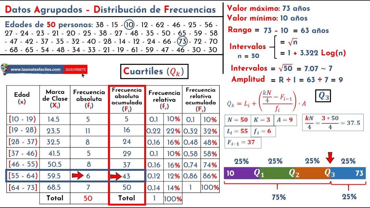
- 🔢 Los cuartiles son valores que dividen un conjunto de datos en cuatro partes iguales, representados por Q1, Q2 (mediana) y Q3.
- 📉 El Q1 se corresponde con el 25% percentile, el Q2 con el 50% percentile (mediana) y el Q3 con el 75% percentile.
- 🎓 Los scores en el percentil 75 significan que el 75% de los individuos tienen puntajes por debajo de ese valor, y el 25% por encima.
- 📚 Los scores estánndarizados, como el z-score, miden cuántas desviaciones estándar un puntaje está del promedio.
- ⚖️ Un z-score de 0 indica que el puntaje está al mismo nivel que el promedio, mientras que valores positivos y negativos indican desviaciones por encima o por debajo del promedio, respectivamente.
- 📉 Un z-score de 1 significa que el puntaje está una desviación estándar por encima del promedio, y así sucesivamente.
- 🚫 Por convención, los puntajes con z-scores menores de -1.96 o mayores de 1.96 se consideran inusuales o extremos en una distribución normal.
- 💡 Los z-scores pueden ayudar a comprender la posición relativa de un puntaje dentro de una distribución, lo cual puede ser útil para educadores y analistas de datos.
Q & A
¿Qué son los percentiles y cómo se definen?
-Los percentiles son valores que dividen un conjunto de observaciones en 100 partes iguales o puntos en una distribución por debajo de los cuales un cierto porcentaje de los casos yacen.
Si un individuo obtiene un puntaje del 33%, ¿qué significa esto en términos de percentiles?
-Un puntaje del 33% en el 50º percentile indica que el 50% de las personas obtuvieron un puntaje menor que 33.
¿Cómo se interpreta el 75º percentile en el contexto de un puntaje del 73%?
-El 75º percentile significa que el 75% de las puntuaciones son menores que 73, y el 25% son mayores.
¿Qué son los cuartiles y cómo se relacionan con los percentiles?
-Los cuartiles son valores que ordenan los datos en cuatro partes iguales. El primer cuartil es igual al 25º percentile, el segundo (mediana) al 50º, y el tercero al 75º percentile.
Si un puntaje es igual al segundo cuartil, ¿qué significa eso?
-Si un puntaje es igual al segundo cuartil, significa que está en el 50º percentile o mediana, y que el 50% de los puntajes están por debajo de ese puntaje.
¿Qué es un puntaje de desviación estándar y cómo se calcula?
-Un puntaje de desviación estándar, o z-score, indica cuántas desviaciones estándar un puntaje está del promedio. Se calcula restando el promedio y dividiendo por la desviación estándar.
¿Cómo se interpreta un z-score de +2 en el contexto de una distribución de puntajes?
-Un z-score de +2 indica que el puntaje está a dos desviaciones estándar por encima del promedio.
¿Qué convención se sigue para considerar un z-score como inusual o extremo?
-Por convención, los z-scores menores de -1.96 o mayores de 1.96 se consideran inusuales o extremos, ya que representan los 5% más extremos de la distribución.
¿Cómo se pueden calcular los z-scores en SPSS?
-En SPSS, para calcular z-scores se utiliza la función 'Descriptivos'. Se selecciona la variable a analizar y se marca la opción 'Guardar valores estandarizados como variables'.
¿Cuáles son las diferencias entre las funciones 'Frecuencias', 'Descriptivos' y 'Explorar' en SPSS para calcular estadísticas descriptivas?
-Las funciones 'Frecuencias', 'Descriptivos' y 'Explorar' en SPSS calculan estadísticas descriptivas como el promedio y la desviación estándar, pero difieren en que 'Frecuencias' permite calcular percentiles específicos y analizar una variable a la vez, mientras que 'Explorar' permite desagregar una variable por otra.
Outlines

Cette section est réservée aux utilisateurs payants. Améliorez votre compte pour accéder à cette section.
Améliorer maintenantMindmap

Cette section est réservée aux utilisateurs payants. Améliorez votre compte pour accéder à cette section.
Améliorer maintenantKeywords

Cette section est réservée aux utilisateurs payants. Améliorez votre compte pour accéder à cette section.
Améliorer maintenantHighlights

Cette section est réservée aux utilisateurs payants. Améliorez votre compte pour accéder à cette section.
Améliorer maintenantTranscripts

Cette section est réservée aux utilisateurs payants. Améliorez votre compte pour accéder à cette section.
Améliorer maintenantVoir Plus de Vidéos Connexes
11. Los percentiles y los valores de normalidad | DATOS 2.0 MINI

Descriptive Statistics, Part 1
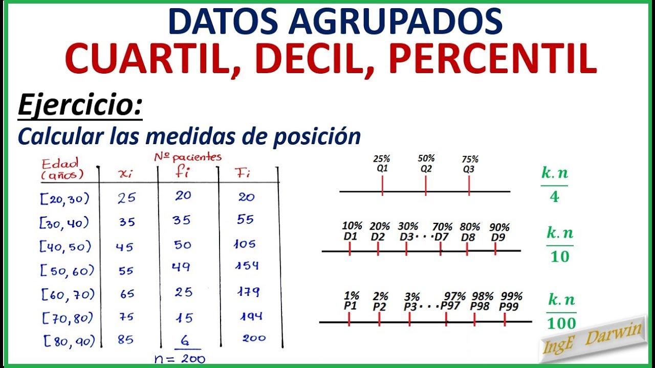
MEDIDAS DE POSICIÓN (CUARTIL, DECIL, PERCENTIL) - DATOS AGRUPADOS
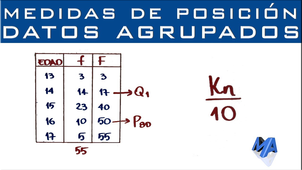
Cuartiles, Deciles y Percentiles | Datos agrupados puntualmente
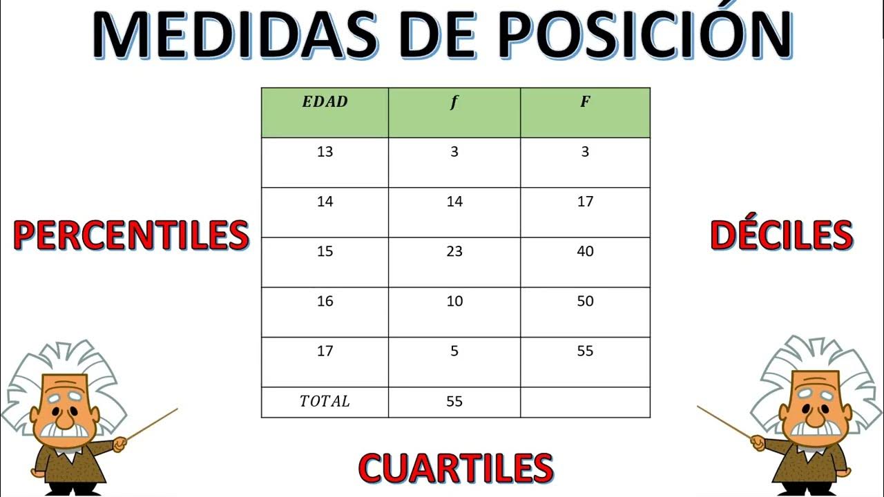
MEDIDAS DE POSICIÓN: PERCENTILES, DECILES Y CUARTILES #estadistica #deciles #percentiles
Cuartiles, Deciles y Percentiles - Datos Agrupados
5.0 / 5 (0 votes)
