EDA - part 1

Develhope
31 Jul 202328:49

Summary

TLDRIn this Python class lecture, the focus is on a practical application of pandas for data manipulation and visualization. The lecturer guides through a real-life case study using a house prices dataset. Key topics include data cleaning, exploratory data analysis, and creating various graphs using matplotlib and seaborn libraries. The session covers handling missing values, analyzing the impact of different features on sale prices, and introduces basic plotting techniques.

Takeaways

  • 📊 This lecture focuses on practical case studies using pandas for data manipulation and visualization with a real estate dataset.
  • 🏠 The dataset explores various factors affecting house prices, emphasizing the importance of data cleaning and exploratory data analysis (EDA).
  • 📈 Visualization is a key component, teaching how to create different types of graphs to represent data insights.
  • 📂 The lecture demonstrates how to import data from a CSV file, emphasizing the use of relative paths for file locations.
  • 🔍 Data exploration techniques such as `head()`, `tail()`, and `shape` are covered to understand the dataset's structure and contents.
  • đŸ§č The importance of data cleaning is highlighted, including checking for and handling duplicates using `drop_duplicates()`.
  • 📊 `describe()` function is used to get an overview of the dataset's statistics, helping to understand data distribution and identify outliers.
  • đŸ•”ïžâ€â™‚ïž The script discusses checking for missing values using `isnull()` and `sum()`, which is crucial for accurate data analysis.
  • 📉 A demonstration on plotting missing values using matplotlib to create bar graphs, showing which features have missing data.
  • 🏡 The lecture explores how to fill missing values, using techniques like filling missing alley types with 'No Alley' as an example.
  • 📊 Grouping data by categories (like Alley, Fence, or Bedroom) and calculating statistics (like mean or median) to find patterns or relationships with the sale price.

Q & A

  • What is the main focus of the lecture series on Python classes?

    -The main focus of the lecture series is to explore practical cases with Python, specifically using the pandas library for data manipulation and visualization.

  • What dataset is used in the lecture for practical case studies?

    -The dataset used in the lecture is about house prices, which depends on a variety of factors, and is intended for data cleaning and exploratory data analysis.

  • How can one obtain the house price dataset mentioned in the lecture?

    -The house price dataset can be obtained from sources like Kaggle or Google Dataset. The lecturer saved a CSV file from the web for the lecture.

  • What is exploratory data analysis and why is it important?

    -Exploratory data analysis (EDA) is the process of using statistics and visualizations to discover patterns in data. It's important for understanding the characteristics of a dataset and informing further analysis or modeling.

  • How does one check for duplicates in a pandas DataFrame?

    -One can check for duplicates in a pandas DataFrame using the `drop_duplicates()` method. This method removes duplicate rows, and if no duplicates are found, the shape of the DataFrame remains the same.

  • What is the significance of checking for null values in a dataset?

    -Checking for null values is significant because it helps identify missing data which can affect the accuracy of statistical analysis. It's a part of data cleaning to ensure the quality of the dataset.

  • How can one visualize the count of missing values in different columns of a DataFrame?

    -One can visualize the count of missing values using a bar plot with matplotlib. The columns can be on the x-axis and the count of missing values on the y-axis.

  • What does the term 'normalize' mean in the context of value counts?

    -In the context of value counts, 'normalize' means to scale the counts to represent proportions rather than absolute numbers, providing a percentage distribution of the unique values.

  • How can one analyze the impact of different parameters on the sale price in the dataset?

    -One can analyze the impact of different parameters on the sale price by using group by operations to calculate statistics like mean or median within categories defined by those parameters.

  • What libraries are mentioned for data visualization in Python?

    -The libraries mentioned for data visualization in Python are matplotlib, seaborn, and plotly.

  • What is the role of seaborn in data visualization compared to matplotlib?

    -Seaborn is built on top of matplotlib and is designed to provide more attractive and informative statistical graphics. It is easier to use for creating complex visualizations and is well adapted for working with pandas DataFrames.

Outlines

00:00

📊 Introduction to Practical Python Pandas Case Study

This paragraph introduces the final chapter of a lecture series on Python classes, focusing on a practical case study using the pandas library. The lecturer recaps the previous lecture on pandas, emphasizing the structure and manipulation of data frames. The current lecture aims to apply these concepts to real-life data, specifically house prices, and introduces the concept of data visualization. The data set is sourced from the internet, likely from platforms like Kaggle or Google Datasets. The lecturer outlines the plan for the lecture, which includes data cleaning, exploratory data analysis (EDA), and various types of graph creation. The process starts with importing necessary libraries and loading data from a CSV file located in a 'Data houses' folder.

05:02

🔍 Exploring and Cleaning the Data Set

The lecturer delves into exploring the data set by using methods like `head()` to view the first few entries and `tail()` for the last entries. The data's structure is examined using `shape`, revealing the number of columns and rows. Attention is given to potential data cleaning tasks, such as checking for duplicate entries using `drop_duplicates()`. The lecturer also discusses the importance of understanding data characteristics using `describe()` to get statistical insights like mean, median, and distribution of values. The data types of columns are checked with `dtypes`, and the presence of null values is assessed with `isnull()`. The paragraph concludes with a discussion on handling missing values, suggesting the creation of a new DataFrame to focus on columns with missing data.

10:03

📊 Visualizing Missing Data with Matplotlib

This section discusses the visualization of missing data using Matplotlib. The lecturer decides to create a bar plot to represent the number of missing values in each column. The process involves using `plt.bar()` to plot the missing values, with adjustments to the figure size for better readability. The lecturer also explains how to rotate the x-axis labels for clarity and adds a title to the plot. Customization options such as changing bar colors and adding labels are also covered. The visualization aims to show the count of missing values across different columns in the DataFrame.

15:07

📈 Handling Missing Values and Initial Data Exploration

The lecturer continues with strategies for handling missing values, often found in columns like 'PoolQC', 'MiscFeature', and others. They demonstrate how to fill missing values with a specific value using `fillna()` and discuss the implications of such actions on data analysis. The exploration of the data set progresses with looking at unique values and their counts using `value_counts()`, with a recommendation to use `normalize=True` for large data sets. The lecturer also touches on grouping data by certain features to analyze average sale prices and how different characteristics like 'Alley', 'LotShape', and 'LandContour' might affect these prices.

20:09

🏡 Analyzing Sale Prices and House Characteristics

The focus of this paragraph is on analyzing how house characteristics like the type of alley, fence, and number of bedrooms might influence sale prices. The lecturer uses group by operations to calculate the average sale price within different categories and discusses the insights gained from these calculations. For example, houses with a 'Paved' alley seem to have higher average sale prices compared to those with 'Gravel' alleys. The exploration also includes looking at the distribution of sale prices relative to the number of bedrooms, suggesting that the number of bedrooms may not have a straightforward correlation with sale price.

25:09

📈 Further Data Exploration and Upcoming Graphing Techniques

In the concluding paragraph, the lecturer summarizes the data exploration done so far, emphasizing the importance of asking the right questions and looking for meaningful patterns in the data. They also provide a sneak peek into the next part of the lecture, which will cover various graphing techniques in Python using libraries like Matplotlib, Seaborn, and possibly Cboard. The goal is to move beyond simple plots to create more complex and informative visualizations that can help in understanding the data better.

Mindmap

Keywords

💡pandas

Pandas is a powerful data manipulation and analysis library in Python. It provides data structures and functions needed to manipulate structured data, making it easier to convert data into a usable format for analysis. In the video, pandas is used to manipulate a dataset of house prices, demonstrating how to load data into a DataFrame, check for duplicates, and perform exploratory data analysis.

💡DataFrame

A DataFrame is a 2-dimensional labeled data structure with columns of potentially different types. It is one of the primary data structures used in pandas for organizing and storing data. The video script mentions the structure of a DataFrame and how it can be manipulated to analyze house prices, such as checking the first few lines with `head()` or the shape of the data.

💡visualization

Visualization refers to the graphical representation of data to understand and communicate insights effectively. The script discusses adding a layer of visualization to the data analysis process using graphs, which helps in interpreting patterns and trends in the house price dataset more intuitively.

💡exploratory data analysis (EDA)

Exploratory Data Analysis (EDA) is the process of using statistics and visualizations to discover patterns within data. In the context of the video, EDA is used to explore the house prices dataset, involving data cleaning and analysis to understand the factors affecting house prices.

💡CSV

CSV stands for Comma-Separated Values, a widely used file format for storing tabular data. The script mentions saving a CSV file from the web, which is then loaded into a pandas DataFrame for analysis. CSV files are a common data source for pandas operations.

💡data cleaning

Data cleaning is the process of detecting and correcting (or removing) corrupt or inaccurate records from a dataset. The video script refers to checking for duplicates in the dataset as part of the data cleaning process, which is crucial for ensuring the accuracy of the analysis.

💡matplotlib

Matplotlib is a plotting library in Python used for creating static, interactive, and animated visualizations. The script describes using matplotlib to create bar plots to visualize the missing values in the dataset, demonstrating how to customize the plot with titles and labels.

💡missing values

Missing values refer to the absence of data in one or more fields in a database or dataset. The video discusses identifying and handling missing values in the house prices dataset, such as checking for null values and deciding how to fill or impute these missing values.

💡normalize

Normalization is a technique used to change the values of numeric levels in a dataset to a common scale. In the script, normalization is mentioned in the context of value counts, where setting normalize to true helps in understanding the percentage distribution of unique values in a column.

💡group by

Group by is a method used in pandas to group rows that have the same value in specified columns. The script uses 'group by' to analyze how the sale price varies depending on certain parameters, such as the type of alley or fence, providing insights into different categories within the dataset.

💡Seaborn

Seaborn is a Python data visualization library based on matplotlib that provides a high-level interface for drawing attractive and informative statistical graphics. The video mentions using Seaborn for more advanced visualizations, suggesting its ease of use and effectiveness for creating informative graphs.

Highlights

Introduction to the last chapter on Python classes focusing on practical case with pandas.

Overview of the lecture's goal: to analyze house prices data set with visualizations.

Explanation of where to find data sets for analysis, such as Kaggle and Google Datasets.

Demonstration of loading a CSV file into a pandas DataFrame.

Use of `head()` to view the first few lines of the data set.

Checking the shape of the data frame to understand its dimensions.

Importance of data cleaning and checking for duplicates.

Using `describe()` to get an overview of the data's statistics.

Checking data types and handling missing values in the data set.

Explanation of how to visualize missing values using a bar plot.

Customizing plot aesthetics like title, labels, and colors.

Strategies for dealing with missing values, such as filling them with a specific value.

Analyzing the distribution of sale prices and its relation to different features.

Using `groupby()` to explore how sale price varies by different categorical variables.

Exploring the impact of features like 'Alley' on the sale price.

Comparing the average sale price across different categories like 'BsmtQual'.

Discussing the importance of asking the right questions during data analysis.

Introduction to the second part of the lecture focusing on graphing in Python.

Overview of different types of plots that will be covered in the lecture.

Transcripts

play00:00

[Music]

play00:05

hello everyone and in this part of the

play00:08

lecture which is the last chapter for

play00:10

the python classes uh we're gonna go

play00:13

about around a practical case with

play00:16

pandas so in the last lecture we've seen

play00:19

how it was looking to work with pandas

play00:21

so we've seen the structure of data

play00:23

frame how we can do how we can

play00:24

manipulate those objects

play00:27

in this part we still couldn't

play00:30

manipulate them in real life so we can

play00:32

rehearse the concept we've already seen

play00:34

basically but we're going to add another

play00:37

layer the other layer is a visualization

play00:40

so we're going to learn how to do graph

play00:43

um we're going to resist along to a real

play00:45

data set so the data set we're going to

play00:47

explore is about some house prices so

play00:51

house prices depends on a variety of

play00:53

things and

play00:56

uh we're gonna explore this data set to

play00:59

some data cleaning see how it works and

play01:01

we're gonna do this data exploration uh

play01:05

data exploration a little nickname

play01:07

foreign

play01:08

exploratory data analysis and we also

play01:11

going to see how to do graph different

play01:13

kind of graph simple one etc etc

play01:17

um so this is how it works uh what data

play01:20

should be used uh so as explained you

play01:23

know uh in another lecture maybe if you

play01:25

did SQL classes we're going to use data

play01:30

that is a part of a horse price data set

play01:32

so to find data you can go on kaggle you

play01:35

can go on Google data set Etc there is

play01:38

lots of data set available

play01:40

so what I did first

play01:42

is I saved this CSV somewhere so I save

play01:47

a CSV file I download it from the web I

play01:50

save it from the website and then I'm

play01:53

able

play01:54

um to see what's happening so this

play01:56

lesson uh we're gonna basically go

play01:59

through a wool notebook so that's okay

play02:01

we're going to throw in a book I'm going

play02:02

to explain how we do graph or we can

play02:04

explain graph and how basically this

play02:06

exploratory data analysis is working so

play02:09

that's the main part of this lecture

play02:11

what is if you want a practical case of

play02:15

what we learned before and how it will

play02:17

look now

play02:18

so uh I created a bit of a skeleton of a

play02:22

notebook right but there is uh other

play02:25

stuff that can be done so I just have a

play02:28

bit of a plan here so uh what we want to

play02:32

do as a goal is we want to analyze our

play02:34

data so we want to analyze our data and

play02:38

first when we start a notebook we need

play02:41

to import some libraries so I import

play02:43

some libraries the one we know for new

play02:45

are this one and this one this one a

play02:47

visual one but I will go back to this

play02:49

Library when we use them

play02:52

um

play02:53

so we can execute it and then

play02:57

I can restart my channel maybe Aristotle

play03:01

so I executed this stuff into restart so

play03:05

it's fresh and then I do DF so to charge

play03:08

my data I use the same as before ifpd

play03:12

that refer to pandas and then I got this

play03:15

dot rate CSV and I save my data in a

play03:18

file in a folder called Data houses

play03:20

slash train CSV so this is a relative

play03:23

path to my CSV file the file is called

play03:29

train.csv and it's in the folder data

play03:31

house so yes this is a relative path

play03:34

from the point of this notebook so let's

play03:36

say if this notebook if my notebook

play03:39

uh so let's say I'm gonna open a

play03:41

markdown cell to explain how it works

play03:45

um so let's say that here activate my

play03:49

keyboard uh so we have this mode on sale

play03:53

um and so let's say I have my documents

play03:56

so let's say it's like this right

play03:57

documents

play03:59

so let's say you have my documents

play04:01

folder and in my documents folder I have

play04:03

this one so my EGR prices so this

play04:07

notebook you know Eda prices

play04:09

Ada process idea prices yeah

play04:13

Eda Eda

play04:16

Eda

play04:17

prices dot e by n b e b so this is what

play04:23

we got right and then I have a folder

play04:24

here

play04:26

that are called Data houses

play04:30

and in this folder in this folder so in

play04:33

the folder

play04:36

I have something that I call train dot

play04:40

CSV

play04:41

so yeah so either price and the folder

play04:44

data houses are in the same

play04:46

um in the same folder if for instance

play04:49

this trained on CSV were there if it's a

play04:52

data what there then I will remove this

play04:54

data horses.train right because it's the

play04:57

same it's like a relative path

play04:59

so this is how it works my train this is

play05:02

not the case so I have my idea my photo

play05:04

data host and in my photo data host I

play05:07

have this train.csc so I can import this

play05:10

trained on CSV so I have a GF

play05:14

then I want to check how my data is

play05:16

looking like right so there is different

play05:17

thing I can do to check how the data is

play05:20

looking like

play05:21

different uh stuff you can do so

play05:23

remember we can just do dheav.head and

play05:26

then we will get the first five line so

play05:28

we can get a bit you know like

play05:31

um

play05:33

checking what is my data looking like so

play05:36

you have an index I have simpler so need

play05:38

lot Frontage area there is some

play05:42

situatives I think this is a type of

play05:43

straight if it is in La if it wizard

play05:46

shape is there is a contour is there is

play05:48

like some pool some utilities some fence

play05:51

so you have lots of features for the

play05:53

horses and then you get to sell

play05:55

condition normal abnormal and you get

play05:57

the same price

play05:58

to in this analysis what we're

play06:00

interested at is a sale price and we're

play06:02

interested at or how the sale price vary

play06:04

depending on some parameter right so we

play06:07

do see we have a lot we don't know all

play06:09

of them what it means

play06:11

um but we know that there is also a

play06:13

description file that is provided with

play06:15

the data I'm not showing it here because

play06:17

I don't want to just speak about it that

play06:19

I will speak about the color and that

play06:20

makes sense when we look at them more or

play06:22

less

play06:23

uh so this is how we can check how the

play06:26

data is looking like with this head and

play06:28

remember by default is the five first

play06:30

line if I want to see the top 10 iPad to

play06:33

10 here and I'm able uh to see more

play06:35

stuff there is also these functions that

play06:37

we call tail and uh tail uh we able to

play06:41

see the tail so the last one another

play06:43

stuff I can do

play06:45

um to check or with my data I could look

play06:48

at the shape right so I could do the F

play06:50

shape and I can see that I have 81

play06:51

columns so I have 80 features

play06:54

um I mean there is a IG colon and a

play06:56

sales price column so maybe 79 features

play06:59

that I will look at and I have 1460 row

play07:02

so as it says answering the question how

play07:04

much data you know

play07:06

and then I'm like either replicates you

play07:09

know so how do I do I can check drop

play07:11

duplicates these are duplicates in my

play07:13

data they say it's part of the data

play07:14

cleaning you know if I was having here a

play07:17

data cleaning part

play07:18

this is what I will do you know first

play07:20

you know I would check for duplicates

play07:21

why because if then I do some counts and

play07:24

I'll do some

play07:25

um

play07:27

um if I do some a statistic if I have

play07:29

duplicates it's not going to be accurate

play07:31

right so I can do drop duplicates and I

play07:34

do dot shape right so if I get a new

play07:37

data frame and it has the same shape as

play07:39

before I know that will not be duplicate

play07:40

so if I drop the duplicate for my data

play07:43

frame I got the same shape as before

play07:45

meaning I have no

play07:48

um no duplicate rows so it happens

play07:50

sometimes we have duplicates when for

play07:52

instance

play07:54

um you you start

play07:56

with a data there is a process that is

play07:59

filling your data and there is a fail

play08:00

somewhere and then you restart it and

play08:02

you have data duplicate so this is some

play08:04

things that could happen or you save it

play08:07

twice or you concatenate some stuff so

play08:10

yeah there is reason why they could have

play08:11

duplicate uh you just have twice

play08:14

whatever or you merge in a different

play08:17

stuff so yeah copies that you have

play08:19

duplicates so you just want to check how

play08:21

it works then we might want to check you

play08:25

know the characters stick in the data so

play08:27

relax maybe there is

play08:30

um

play08:33

so this is something or we can check the

play08:36

characteristic so we can do uh describe

play08:39

up so we can do describe and we can see

play08:42

that we have 460 we have a mean for the

play08:45

ID we can see like the lot area on

play08:48

average it's like 10 000 accuracy so

play08:50

meter Square maybe uh it's close to the

play08:54

median and we see like

play08:56

um half like from this one to this one

play08:59

75 of them are below 11 000 so you know

play09:03

like 75 of them are like still close to

play09:06

the average right the average between 10

play09:08

000 but you got like very huge

play09:10

disparities if you look at the lottery

play09:12

then you get the conditions or you're

play09:14

built so in average it's 2071 and the

play09:18

most recent houses are constructing

play09:20

tougher 2010.

play09:22

and you get something and you if you're

play09:24

interested in the sale price because

play09:25

it's a colon we're interested in we do

play09:28

see that the average it's like 80k and

play09:30

uh the most expensive one are like less

play09:33

than a million still or yeah uh one two

play09:36

three yeah it's less than me 700k

play09:39

um yeah so this is a possibility for uh

play09:43

this house prices and this is if you

play09:45

want a bit uh so overview we have uh on

play09:49

it

play09:51

um then as I read something else we can

play09:53

check the data type so we can use this

play09:55

like d-types so we have different

play09:56

columns uh yeah

play09:58

his parents as and we can see that we

play10:01

have some integers that we have some

play10:03

objects uh but most of them are like

play10:05

intake when it's like an object usually

play10:07

it means like you know it's like usually

play10:09

it's a string or there is a missing a

play10:11

mix for instance so the cell type is

play10:16

um if we remember I think cell type is

play10:19

like a lot of NR or series like yeah

play10:21

lots of like string like text so in this

play10:24

case it will be an object it's only

play10:26

integer if everything in the colon is an

play10:28

integer then it will return an intake

play10:30

then we can also check the null value

play10:34

you know we're like

play10:35

is there some value missing so you do

play10:38

see here is that in like fans

play10:40

miscellaneous features miscellaneous

play10:42

values Etc we do have a lot of like a

play10:45

lay none babe Etc we do have a lot of

play10:48

um values that are missing you like it

play10:50

does it represent a lot you know so I'm

play10:53

going to check some null value so for

play10:54

this I have my DF and I can do easy so

play10:57

remember when we do is an a I check for

play11:00

every

play11:01

um

play11:03

entity like row and colon every element

play11:06

a mic table if it's not and then I do a

play11:09

true or false and then if I do a sum

play11:12

it will sum per column so I will see

play11:14

that for first sum it will be a lot for

play11:18

over node

play11:20

um so

play11:21

this is important to do at first uh why

play11:26

because it's important to know what

play11:28

value I'm missing for instance and then

play11:32

we can check uh what to do with the

play11:36

missing value right why are some value

play11:39

missing so for this uh we're gonna go

play11:43

through a college so you know we have if

play11:45

we do df.colon we have all the possible

play11:48

colon here so we see there is all this

play11:51

possible currents and we like well

play11:55

um

play11:56

maybe we can check

play11:58

what's values are missing and I want to

play12:00

check which one are the missing value so

play12:03

for this uh first

play12:05

um I want to get the ones that are

play12:07

missing you know so I'm going to create

play12:08

a data frame where um I got values that

play12:12

I'm missing so missing I have my DF

play12:15

let's say I have my DF and I have my

play12:17

izenae and I do my sum so this is what I

play12:20

made before and this is going to be my

play12:22

missing

play12:24

so missing is going to look like bits

play12:27

like a data frame right

play12:29

so missing is a bit like this index with

play12:31

a colon I think

play12:33

um and then I'm gonna do missing and I

play12:35

just want to get one where I got missing

play12:37

value right if I have zero I'm not

play12:38

interested in it so here I got my

play12:41

missing

play12:43

I'm not oh quite interesting you know I

play12:45

see that there is a lot of fans

play12:47

miscellaneous feature pool fireplace

play12:50

that stuff and I'm like well I would

play12:52

like to sort my values right I can do

play12:54

sold values if I do sweet values here

play12:56

yeah so one was only one missing which

play12:59

is electrical and I have the one with a

play13:01

lot of stuff what does it mean when I

play13:03

got a lot of this missing value uh when

play13:06

I got a lot of this missing value it

play13:08

mean

play13:09

um that you know maybe it's not

play13:10

specified if I'll have pool QC maybe

play13:12

just mean I don't have a pool you know

play13:14

so I can go here in my pool

play13:17

maybe a heavy due and I see that well

play13:19

maybe if I have pull it just means zero

play13:21

I don't have it you know so I'm like

play13:23

okay I want to look at you know the

play13:25

value for the pool so I'm going to be

play13:27

like df.pull

play13:29

DF dot pull QC

play13:31

up and I'm looking like unique so if I

play13:34

do dot unique I would like the unique

play13:36

value you know so either I got nothing

play13:38

here are things there's exterior

play13:41

um in the ground or something like that

play13:43

so I have like different value for the

play13:46

description of my pool if I have Ali I

play13:50

do see that Ali unique gravel or paved

play13:54

and none meaning uh if I have nothing

play13:57

meaning I have just no Ali so if there

play14:00

is no Ali I can't specify if it's paved

play14:02

or not basically

play14:04

so this is it so we're gonna go through

play14:07

our first uh plot so here we know we

play14:10

have missing value and we would like to

play14:12

represent this value as a bar so we

play14:14

would like this to be the abscess and

play14:16

this value to be the colon in the bar so

play14:18

for this we will use

play14:20

um a library called multiple clip so

play14:22

matplotlib is a library that we imported

play14:25

here so here we did import

play14:27

matplotlid.pi plot as PLT so now we're

play14:30

going to use this PLT that we have here

play14:32

to plot the graph so here you have this

play14:34

missing salt values so what I want to do

play14:37

I have my PLT I do dot bar because I

play14:40

want a bar plot so I want a bar plot and

play14:43

I want to get my media I want to plot

play14:45

this I will block this it's interesting

play14:48

okay

play14:50

yay Heights Dodge index

play14:54

so if I do dot index here

play14:57

I will have the value here right and if

play15:00

I do dot values

play15:02

I will have my values so my abscess if I

play15:06

do my index is going to be this so here

play15:10

um when I do my plt.bar I have to

play15:12

specify your X and eight so an abscess

play15:15

and the node in it so here this would be

play15:17

my abscess and then I did my ordinate so

play15:22

when I did my ordinate I put here my

play15:24

values

play15:25

so this is how it works and here as you

play15:28

see uh I have uh something like this but

play15:32

I see here that I don't have you know

play15:35

they're all stuck together so what I can

play15:38

do two possibilities I can say to my

play15:41

figure to be bigger you know so I say

play15:44

prt.figures this means I'm going to

play15:46

create a figure

play15:48

and my figure is having some

play15:49

particularity so my figure is having

play15:52

some particularity let's say I can say

play15:54

which size I want so if I put 15 5 mean

play15:57

it's going to be 15 long length and like

play16:00

five of eight so if I do this well I do

play16:04

see this a bit better right because uh

play16:06

you know I'm able to read them a bit but

play16:08

it's still difficult so I'm like oh can

play16:11

I do this you know so there is in PLT so

play16:14

PLT is a celebrity that we use uh first

play16:17

to trace graph there is something called

play16:19

egg sticks

play16:21

so there is you know different stuff

play16:22

that you can hear and extens so xdx is

play16:26

referring to the ticks on the x-axis so

play16:29

this is in graph so x-axis and this is

play16:32

the y-axis so I have my X text and what

play16:35

I want to do is I want to rotate the

play16:38

rotation

play16:41

um and I want to rotate my X text so

play16:44

here they are flat and if I rotate them

play16:46

from an angle of 90 degrees I look like

play16:48

this

play16:50

to avoid all this kind of real with

play16:54

return we can just do PLT and we've said

play16:57

PLC dojo we have our figure so here we

play16:59

do see that the most less mystical

play17:02

feature with some missing value but not

play17:04

too much electrical and the one with

play17:07

most are something like fence Ali pool

play17:09

miscellaneous feature Etc

play17:13

um so here we have and relax well maybe

play17:15

I want to put the title so to put the

play17:17

title I will do plt.title and I will put

play17:19

a string so I will put a string and I

play17:21

will say what is my graph show me what

play17:24

is my graph showing uh to answer the

play17:26

question my graph is showing a missing

play17:29

value in the different color so we're

play17:31

gonna say count of missing values in our

play17:36

data frame

play17:39

you know that right yeah and then we do

play17:42

see this is here uh this uh PLT dot

play17:46

title a bit like method you know you can

play17:47

specify other stuff you could put like

play17:50

uh something like font size

play17:54

I think not fondact and then you will

play17:58

put maybe like Ariel you know or real I

play18:01

don't know if it exists uh no no like

play18:05

but yeah you can get the contact or like

play18:08

some font size Etc or you can also

play18:10

change colors so let's say you want to

play18:12

change the colors where would you go

play18:14

let's say you want your bar to have

play18:15

another color you will go there and you

play18:17

will add this is this line is producing

play18:21

the bar you remember we did it together

play18:22

and let's say I want to color a red I

play18:25

will do color equal red and then it will

play18:27

be red if I want the color to be green

play18:30

here I go there but if I want if there

play18:33

is a color that is like not known it's

play18:35

gonna have a mirror right and it's going

play18:37

to be the color has to be pasted as a

play18:39

list uh so I'm like okay I know

play18:42

um I'm gonna put purple purple purple

play18:48

as color you can also provide like AGB

play18:52

values you get also uh provide a HTML

play18:56

and X called and stuff so you can really

play18:58

provide uh in Python lots of stuff so

play19:01

your graph are customizable you can add

play19:04

um label as well right so I create my

play19:06

stuff I'm like okay I need my Legend to

play19:08

be turned this is about the X text and I

play19:11

can add a title and I can also add a

play19:14

label so I can also add xlabel and my X

play19:17

label is like what is there so what is

play19:20

there is like Columns of my data frame

play19:22

on the x-axis right Columns of the data

play19:26

frame so this is my Columns of the data

play19:28

frame and we do see it there and then I

play19:31

have my PLT I'm going to do dot y level

play19:34

y level I mean it's it's clear from the

play19:37

title that is a count of missing value

play19:39

but to show you I'm still going to show

play19:41

you how this is working so I have my PLT

play19:44

label uh and for this plg label we're

play19:48

gonna put count of missing value so we

play19:51

put count off missing value there so we

play19:54

have this uh so here we have

play19:57

um total graph with like a title we are

play20:00

able to manage you know this like

play20:02

different X text

play20:04

and we have this column of the data

play20:06

frame control of missing value etc etc

play20:08

so this is how it works so uh what to do

play20:12

with the missing value so most of the

play20:14

time and I mean lacks of subjected fiber

play20:16

attribute like missing pool fans no

play20:18

garage and basements uh so yeah so we do

play20:22

see

play20:22

um that we we could like let's say I

play20:25

want to put zero you know for instance

play20:27

uh nothing no offense so let's say you

play20:30

know you remember we're having all like

play20:32

a filene so what I could do is I could

play20:35

do the if dot filene I know which uh

play20:38

what I want to do you know so you could

play20:40

do like Oh I wanna name how I want to

play20:43

feel my particular value so you could

play20:46

have you want a subset you know you

play20:48

don't have uh when you do a feeling a

play20:52

um

play20:53

to uh to do your stuff so two different

play20:56

stuff either you could do DF dot

play20:59

Ula so it would fill a name with like no

play21:02

Ali

play21:03

and then if you do you dot value counts

play21:07

let's say value counts

play21:10

up

play21:15

so we see like most of the

play21:19

um stuff in data frame I have no Ali you

play21:21

could normalize as well

play21:23

up normalize equal true and you see like

play21:25

in 93 of the cases there is no alley in

play21:28

three percent of the case says I have

play21:29

gravel and in only 2.8 percent of the

play21:31

case uh the alley is baked

play21:34

um yeah so this is how it works this is

play21:36

not filling my array because I haven't

play21:39

say I haven't say like uh this in place

play21:41

equal true etc etc right if you put the

play21:44

implicit called true it would change if

play21:46

you don't put the implicit control you

play21:48

create a new object and then you have to

play21:49

change old object if you want or you

play21:51

just copy your new data frame Etc these

play21:54

are all the stuffs that are I will say

play21:57

yeah possible

play22:00

um so this is it to do the stuff uh here

play22:03

we do see a different colon

play22:06

um then uh something else that we're

play22:08

interested at is how much the sale price

play22:11

is

play22:12

um let's say varying right

play22:15

um soon

play22:17

um we could you look at the unique value

play22:21

in a colon right so here that's what we

play22:23

do when I was doing this dot unique you

play22:26

can look what are the different

play22:28

possibilities when you do a value counts

play22:30

you have more than the three

play22:32

possibilities right you have bitless

play22:34

repartition for big data set I recommend

play22:37

using this normalizer called true

play22:39

because it gives you a better picture

play22:40

you already know your data set is 1400

play22:43

there is thousand four hundred rows so

play22:45

there's no duplicates and then if you do

play22:48

this like dot value counts you will have

play22:50

access to all the different values the

play22:52

different unique values that I'll take

play22:54

on in this column and then you know the

play22:56

percentages so you know how it is

play22:58

reported

play23:00

um yeah

play23:02

um so what we can also look at if we do

play23:05

some data exploration is you know I'm

play23:07

interested into this alley that I feel

play23:09

with no Ali and I'm like or as I said is

play23:12

the sales page the sales price

play23:15

average surprise

play23:16

um defer within those groups you know so

play23:19

I'm having this and I'm like okay I have

play23:21

this Ali

play23:23

um and what I want to do is I want to

play23:25

group my DF pies up so I'm doing what I

play23:27

have my DF and I do group by

play23:29

so why do group by but here you know I

play23:32

was having only value with my La so I'm

play23:34

grouping by this

play23:36

Ali but this is another stuff we can do

play23:39

and earlier I'm like okay I'm interested

play23:41

in what I'm interested in my sales price

play23:44

and I want to see if my sale price

play23:46

um is going to vary depending on this

play23:49

characteristic

play23:50

uh surprise dot mean yeah I need to

play23:53

close the parentheses

play23:56

Group by closer parenthesis no brackets

play23:59

set price that mean and here I do see

play24:03

that if there is no Ali I'm like

play24:07

1800k and here I'm like 122 and 160. so

play24:12

it looks like when there is a gravel

play24:14

array it's like which represent a pave

play24:16

one for instance and then I say but you

play24:19

also look like there's only two and

play24:20

three percent so it's not very like a

play24:22

wooden comparison no Ali with the two

play24:24

other one but because it's two one at

play24:26

two percent we're like okay maybe pave

play24:28

is better than gravel and I guess maybe

play24:29

it's more expensive or something so

play24:31

justifies the house uh to be good like

play24:34

if you have a good looking house maybe

play24:35

you're not just going to put gravel in

play24:37

there so this is something very good

play24:40

it's like group by to check what the

play24:42

difference price you know we can check

play24:44

um if the one with like uh the fans are

play24:48

more expensive so to do that I can do

play24:50

the same thing with the fence so to do

play24:52

the same thing with the fence I will do

play24:54

DF Group by

play24:57

um let's say I have my fence I think it

play24:59

exists and I can do dolceprice.min so I

play25:03

would grow up by the unique value of

play25:04

fans and then I have master and I do see

play25:07

that where there is a bit of variations

play25:09

this one are closed and this one with

play25:11

the GDP I don't know what it means uh

play25:14

but has a bit more expensive stuff

play25:17

uh the one that is a bit more

play25:19

interesting to look at is a bedroom

play25:21

average so this is

play25:24

um if we look at this bedroom average so

play25:27

we do see that

play25:29

um

play25:30

upper bedroom average here if I do a

play25:34

value count on this we do see that we

play25:37

have like three two one so it's like the

play25:39

number uh of a bedroom I guess or the

play25:43

bedroom yeah the group yeah so if I do a

play25:46

DF Buy sales price and then what I want

play25:49

to do I want to solve the index right so

play25:52

I want to sort index so here we'll have

play25:54

the room with zero and then the room

play25:56

upper so I do see that there is

play25:59

um some I always say dissimilarities

play26:02

um and that you know okay so one with

play26:04

eight uh is as expensive as the one with

play26:07

like four here so we do see there is not

play26:09

very a correlation like or something we

play26:11

can explain with just like bedroom

play26:12

average great size

play26:15

um Enzo index

play26:16

uh soon uh for this part we've and we

play26:21

mainly do like exploration so this is

play26:24

like group by uh mean uh so we're

play26:26

interested uh what is interesting at us

play26:28

in the study is to interest uh whether

play26:31

this interest in the sales price and we

play26:33

want to see how different parameters of

play26:34

an influence of it so doing this like

play26:36

group by and then looking at like oh is

play26:39

the average is different within

play26:41

categories is a good stuff to start to

play26:43

data analysis you know you'll have

play26:44

different parameters and you're like oh

play26:46

is the behaviors the same in different

play26:48

groups right

play26:49

um You can not only look at the median

play26:51

but you can look at you know the median

play26:53

and then you will look at the median and

play26:55

maybe it's more interesting for you to

play26:57

look at the median price or you can look

play26:59

maybe at the mean you know how is the

play27:00

cheapest house doing in all of this

play27:02

category uh and you can also look by

play27:05

bedroom average or the Ali you know so

play27:08

there is lots of different stuff you can

play27:09

do and in this case it's really you

play27:12

asking you a question you know what am I

play27:14

interested to see what is interesting

play27:17

for me to see here so this is main

play27:19

question you should ask yourself what is

play27:21

interesting for me to see there uh what

play27:23

question I want to answer yeah I'm like

play27:25

okay is this parameter having an

play27:26

importance of the sale price on average

play27:29

so I'm looking at the mean

play27:32

which is a good indication you know of

play27:34

like how it's reported I can look at the

play27:36

STD does it vary a lot uh above within

play27:40

the categories so this is uh something

play27:43

very typical and nice to do

play27:46

um

play27:47

then in the second part of this lecture

play27:49

we're more gonna see how to do the graph

play27:51

in Python so some basic plots and then

play27:55

we're going to do some plot plot with

play27:57

time series do some histogram and then

play28:00

do this data exploration so this is what

play28:03

we're going to do just after this in the

play28:06

graph so I'm going to explain you how

play28:08

you can build a graph with PLT that we

play28:11

already see here a bit how it was

play28:13

working but we're going to see more way

play28:14

of doing it not only about plot but all

play28:17

the kind of plot and then we will use

play28:19

another Library called Seaborn and when

play28:22

using Seaborn are you going to see how

play28:24

rich it is and how I I think it's like

play28:27

one of the good library to start with

play28:29

because it's very that pipelot to start

play28:31

and then build on top top of Pi plot you

play28:35

have C board and cboard is very complex

play28:37

you can do very complex graph and C bone

play28:40

is very adapted to data frame to do

play28:43

graph for instance

play28:44

[Music]

Rate This
★
★
★
★
★

5.0 / 5 (0 votes)

Étiquettes Connexes
PythonData AnalysisPandasVisualizationData CleaningExploratory Data AnalysisEDAGraph PlottingData ScienceMachine Learning
Besoin d'un résumé en anglais ?