Image Processing on Zynq (FPGAs) : Part 1 Introduction
Summary
TLDRThis tutorial series introduces image processing on FPGAs and Zynq chips, focusing on grayscale and color images as two-dimensional arrays. It differentiates between point processing, where output pixels depend solely on corresponding input pixels, and neighborhood processing, which considers neighboring pixels for output values. The architecture involves streaming images from DDR memory to an IP core via a DMA controller. The tutorial also covers convolution operations using kernels and the challenges of processing image edges. It discusses system design considerations, including buffering strategies and the use of line buffers and multiplexers for efficient processing. The series will progress to coding and implementation on FPGAs.
Takeaways
- 📚 The tutorial series will cover image processing on FPGAs and Zynq chips, with a focus on practical application rather than theoretical details.
- 🖼️ Images are described as two-dimensional arrays, with grayscale images being 2D and color images typically 3D arrays, where each element represents a pixel.
- 🔄 Image processing is divided into point processing and neighborhood processing, with point processing involving transformations that depend solely on the value of a single pixel.
- 🔀 In point processing, operations like image inversion can be performed by simple transformations such as 255 minus the input pixel value.
- 🌐 For system design in image processing, images are initially stored in external DDR memory and then streamed to the processing IP via a DMA controller.
- 🔄 Neighborhood processing involves considering the pixel's neighbors for operations, which can include different types of neighbors and convolution with a kernel.
- 🛠️ Hardware implementation for neighborhood processing requires buffering parts of the image within the FPGA due to non-consecutive pixel processing needs.
- 💾 Line buffers are used to store parts of the image within the FPGA, and multiplexers are employed to intelligently reuse lines for efficient processing.
- 🔗 The tutorial discusses the importance of parallelizing data transmission and processing to improve system performance, such as adding extra line buffers.
- 🛡️ Interrupt-based processing is mentioned as a method to handle data streaming between the IP and the PS, with an interrupt service routine to manage data flow efficiently.
Q & A
What is the main focus of the tutorial series mentioned in the transcript?
-The tutorial series focuses on image processing on FPGAs and specifically on Zynq chips.
Which textbook is recommended for detailed information on image processing?
-For detailed information on image processing, the transcript recommends 'Digital Image Processing' by Gonzalez.
How are images represented in terms of data structure?
-Images are represented as two-dimensional arrays or matrices. Grayscale images are typically one-dimensional arrays, while color images are three-dimensional arrays with RGB values for each pixel.
What are the two broad categories of image processing mentioned in the transcript?
-The two broad categories of image processing mentioned are point processing and neighborhood processing.
How does point processing differ from neighborhood processing?
-In point processing, the value of a pixel in the output image depends only on the corresponding pixel in the input image. In contrast, in neighborhood processing, the value of a pixel in the output image depends on the pixel and its neighboring pixels in the input image.
What is an example of a point processing operation discussed in the transcript?
-An example of a point processing operation is image inversion, where the pixel value in the output image is calculated as 255 minus the pixel value in the input image.
How is the image data transferred from external DDR memory to the image processing IP in the described architecture?
-The image data is transferred from external DDR memory to the image processing IP using a DMA controller, which is configured by a driver running on the processor.
What is the role of line buffers in the neighborhood processing architecture?
-Line buffers in the neighborhood processing architecture are used to store parts of the image necessary for processing. They allow for the buffering of image lines to facilitate the convolution operation with a kernel.
Why is pure streaming architecture not suitable for neighborhood processing?
-Pure streaming architecture is not suitable for neighborhood processing because the pixels being processed are not consecutive. The convolution operation requires specific groups of pixels that may not be in sequential order.
What is the purpose of multiplexers in the line buffer architecture?
-Multiplexers in the line buffer architecture are used to intelligently select and reuse the correct line buffers for the convolution operation, ensuring that the same line is not unnecessarily fetched multiple times from external memory.
How does adding a fourth line buffer improve the system performance in the architecture?
-Adding a fourth line buffer allows data transmission and processing to happen in parallel, reducing idle time and improving overall system performance by enabling continuous data flow and processing without waiting for one operation to complete before starting another.
What is the significance of the interrupt-based processing mentioned in the transcript?
-Interrupt-based processing is significant as it allows for efficient communication between the IP and the processor, enabling the processor to send the next line of data to the IP as soon as a convolution operation is completed, thus maintaining a smooth and continuous processing workflow.
Outlines
🖼️ Introduction to Image Processing
This paragraph introduces a tutorial series on image processing, specifically focusing on FPGAs and Zynq chips. It suggests referring to a standard textbook, such as 'Digital Image Processing' by Gonzalez, for detailed information. The tutorial is divided into multiple parts, starting with an introduction to the theory of image processing. Images are described as two-dimensional arrays, with grayscale images represented by single-byte intensity values and color images by three RGB values. The paragraph categorizes image processing into point processing, where output pixel values depend solely on the corresponding input pixel, and neighborhood processing, which will be detailed in subsequent parts. The architecture for designing a pixel processing system is briefly mentioned, involving interfacing with a DMA controller and processing images stored in external DDR memory.
🔍 Neighborhood Processing in Image Processing
Paragraph 2 delves into neighborhood processing, a technique where the value of a pixel in the output image depends on its neighbors in the input image. It explains that different types of neighbors can be considered, from immediate to more distant ones, and that this typically involves a 2D convolution with a smaller matrix known as a kernel. The process involves multiplying values in the kernel with corresponding pixels in the image and accumulating the results to form the output image. The paragraph also addresses the challenge of processing edge pixels, which may not have the full complement of neighbors, and suggests solutions such as adding dummy rows or reducing the output image's resolution. The hardware implementation of neighborhood processing is also touched upon, noting that it cannot use a pure streaming architecture due to the non-consecutive nature of pixel processing.
💾 Buffering and Processing in Hardware Design
Paragraph 3 discusses the practicalities of buffering and processing images in hardware design for neighborhood processing. It explains that buffering the entire image is impractical due to memory constraints in FPGAs, so only parts of the image necessary for processing are buffered. The concept of line buffers is introduced, which are small memories used to store one line of an image. The paragraph describes how line buffers and multiplexers are used to efficiently reuse the same line buffer multiple times during convolution operations. It also mentions the importance of the order of lines in convolution and how multiplexers are used to select the correct lines. The idea of adding a fourth line buffer to improve system performance by allowing data transmission and processing to occur in parallel is introduced.
🛠️ System Architecture and Interrupt-Based Processing
The final paragraph outlines the system architecture for image processing, emphasizing the use of interrupt-based processing to improve efficiency. It describes a process where images are initially stored in DDR memory, and the DMA controller is configured to stream data to line buffers within the FPGA. Convolution operations are performed, and upon completion of each row, an interrupt is sent to the processor. An interrupt service routine then sends the next line of data to continue the convolution. This process repeats until the entire image is processed. The paragraph also mentions that after convolution, the processed data is streamed back to the DMA controller and then returned to DDR memory. The architecture includes line buffers, multiplexers, and an interrupt mechanism to ensure that data transmission and processing occur efficiently and in parallel.
Mindmap
Keywords
💡Image Processing
💡Grayscale Image
💡Color Image
💡Point Processing
💡Neighborhood Processing
💡Pixel
💡DMA Controller
💡FPGA
💡Zynq Chip
💡2D Convolution
💡Line Buffer
Highlights
Introduction to image processing on FPGAs and Zynq chips.
Reference to the textbook 'Digital Image Processing by Gonzales' for detailed image processing techniques.
Images are two-dimensional arrays, with grayscale images represented by one byte per pixel and color images by three values (RGB).
Classification of image processing into point processing and neighborhood processing.
Point processing involves transformations that depend solely on the value of a single input pixel.
Examples of point processing include image inversion and gray level mapping.
General architecture for designing a system for pixel processing, interfacing with a DMA controller.
Image data is streamed from external DDR memory to the image processing IP via a DMA controller.
The IP processes pixels based on data width, which can be adjusted for performance.
After processing, the image is streamed back to the DMA controller and then to DDR memory.
Neighborhood processing considers the value of neighboring pixels in addition to the pixel of interest.
2D convolution is used in neighborhood processing with a smaller matrix called the kernel.
Different strategies for handling edge pixels in neighborhood processing, such as padding or reducing output resolution.
Hardware implementation challenges for neighborhood processing due to non-consecutive pixel processing.
Use of line buffers and multiplexers to efficiently reuse image lines for convolution.
System architecture improvements by adding a fourth line buffer to allow parallel data transmission and processing.
Interrupt-based processing to coordinate data streaming and convolution operations.
Overview of the complete system architecture, including DDR memory, DMA controller, IP, and interrupt service routine.
Transcripts
hello on in a next set of tutorial we
will be finding out how to do image
processing on a PGA's and on Zink chip
in particular so I'm not going into
details of image processing for that you
may refer to in a standard textbook
maybe digital image processing by
gonzales which is a good reference book
and this is going to be a quietly long
tutorial so i am breaking it into many
different parts so this is the
introduction to the image processing
basically the theory part now as you
know images they are nothing but
two-dimensional arrays they are like
matrix of two dimension if they are
grayscale if they are color images
usually we will say they are three
dimension so in this two dimension each
each box here it represents a pixel if
it is a grayscale you usually have one
byte that are representing the intensity
of that pixel if it's a color image each
box will have three values representing
the RGB values of that pixel so broadly
we are classifying image processing into
two one is called the point processing
other one is called the neighborhood
processing in point processing you have
an input image and you do some operation
on that image and you get the output
image now the particular pixel value in
the output image depends on the
particular pixel value on the input
image so you are basically doing some
transformation operation on a particular
input pixel and you get the
corresponding or per pixel so just
remember the value of the output pixel
depends only upon the value of the input
pixel at that corresponding position and
what our transformation operation you
are doing for example we have the
invasion of
so we have already done this in detail
how this is done
so when you are doing the inversion
operation the pixel value on the output
image will be 255 minus the pixel value
in the input image so there are a lot of
other point processing also for example
you have something called gray level
mapping here what you do is you take an
input pixel value and you add a bias to
that pixel value now depending upon
whether the bias is a positive number or
negative number you will get a picture
with increased brightness or you may get
a pixel picture with decrease badness so
these are what we call as spawn
processing now this is the general
architecture we will follow when we
design a system for pixel processing and
we have already seen this architecture
we actually design this IP for doing
image processing inversion operation
basically and we interface with DMA
controller so in this architecture
initially the image will be stored in
the external DDR memory how you get the
image to that external diría depends
upon what kind of interface you have you
may use Ethernet USB PCI Express
high-speed interfaces or if you have the
low speed interface like you what you
can use that also which is we basically
used in our previous tutorial now from
that DDR the image is stream the pixels
are stream to the image processing IP
with the help of the DMA controller so
basically we will have a driver here
running on the processor who will
configure the DMA controller here and it
will basically send the image data from
external ddr2 30 mi controller and from
the it is stream to your IP now your IP
will be processing the pixels depending
upon what is the data weight for example
in our tutorial that whatever it was 32
that means you can process 4 pixels in
and you will process it but not have it
you can make it 8 16 32 64 whatever
width you choose which may improve the
performance depends and you process it
using your IP after you process it you
will stream it back to the DMA
controller and the DMA controller it
will send that process picture back to
the DDR using the AXI 4 interface and
finally that tender processed image is
in the media you can send it to the
external world through your interfaces
or to a display controller do you return
a monitor so in our previous tutorial we
used a UART interface to send it back to
the computer and we or the computer now
the other kind of popular image
processing technique is called the
neighborhood processing now in
neighborhood processing what happens the
pixel value in your output image not
only depends upon the pixel in the
corresponding position in the input
image but also on the neighbors of that
pixel for example if I am processing
this pixel the value of the transponding
pixel in the output depends on this
pixel as well as his neighbors now
neighbors we can have different kind of
neighbors so there are eight immediately
as you can see there are eight of them
but in many cases we have more neighbors
we can take the pixels which are further
away from this pixel also so here we
have eight and these are also neighbors
they are not immediate neighbors so
depends so basically what you are doing
is you will take your input image and
you will be doing a 2d convolution with
a smaller matrix called the kernel so
this is the Maps representation this is
basically multiplication operation this
is your image and this is so-called
caramel you are multiplying them
together and you are adding them
together to make things clearer let me
show this feature so this is your input
image which is a 2d matrix
you will have a smaller matrix called a
mask or a kernel whose size can be three
by three five by five three by five
different size depending upon what
operation you are doing what you will do
is you will multiply the values in the
mask with the corresponding pixel in the
image so here it is a three by five so
you multiply these these these this okay
and after that you add them together so
basically it's the Mac operation
multiply and accumulator operation and
that multiplied and accumulated result
will be the corresponding pixel in the
output image okay so that's what we are
doing here now again I am showing
pictorially assume this is you a picture
this is the mask Here I am taking a
three by three so there will be some
values here in practical case so you
place the mask on the picture and
multiply each cut off funding values add
them and you are actually getting the
output pixel value for this bit so after
that you move the mask by one pixel
repeat the operation and you get the
value for this pixel in the output image
and you keep on doing it you keep on
moving the mask now when you are doing
this you will notice if you want to
calculate the values of these pixel on
the edges of the image you do not have
eight neighbors for example the corner
once they have only three neighbors here
and the other ones on the edges they
have only fine APIs now how to solve
this issue again you can write in both
there are different ways of that you may
assume a dummy row on the top on the
left right and bottom edges also and
this dummy rows and column they may have
value 0 or you may replicate the same
values of the edges here also and you
can do the calculation here that is one
way of doing it
another way is your awkward picture it
will not have values corresponding to
the pixels on the edges so in this case
the resolution of the output picture
picture will be slightly less than the
resolution of the input picture for
example if you have 512 by 512 input
image the output will be 510 by 5/10
because we are neglecting this row this
row and these two corners so draw eyes
there'll be a reduction of 2 pixel
column wise there will be a reduction of
two fits and so you will have 5 10 by 5
okay so that's how we usually solve the
issue of the pixels on the edge now once
you finish this convolution for this
particular row you will move the mask to
the next row again you are not shifting
by 3 pixels although it is a 3 by 3 you
are shifting only by one pixel so keep
that in mind and you repeat it until you
finish convolution of the enter picture
now when you design hardware for doing
this you cannot use pure streaming
architecture here why because in this
particular case the pixels you are
processing they are not consecutive for
example here these 3 pixels are
consecutive but these 3 pixels they are
not consecutive with these 3 pixels so
when I am streaming data from my
external media I'd be always dreaming
like starting from here I will first
stream this entire line then I scream
this entire line so and and so forth so
pure streaming we cannot use because I
need only these 3 pixel these 3 is the
remaining I don't want then I want these
3 then I want these 3 so on and so forth
so pure streaming based implementation
is not possible so you will have to
buffer the image inside your IP before
you start processing now it won't be
practical to buffer the entire image
inside your IP because depending upon
the image size how much memory you need
to buffer it varies again fight will by
fight all grayscale image you need
around 268 of kilobytes
and if you remember inside FPGA we have
something called the block Rams does
more memory blocks which are like 36
khilafat in science it is HPG and we
have look up tables and flip-flops so
you can make a buffers or small memories
using them but the number of B Rams are
quite limited if you check the
particular FPGA we are using there will
be a few hundred theorems usually and if
you use look-up tables and for us to
make this memory which we call as the
distributor it is going to use a
lot of CL base to do it so you won't
have much CL piece left for implementing
the remaining logic so practically we
will never buffer and enter picture
inside the FPGA unless the picture is
really really small otherwise we won't
buffer the entire picture what we will
do is we will buffer only a part of the
image inside our IP which is necessary
for doing the processing so for example
if you are using this 3 by 3 kernel for
processing if I if I buffer 3 lines of
my image inside the FPGA but it is
enough for me to start processing site I
buffer these 3 lines then I use the
kernel to do convolution and I can keep
on moving the kernel until I finish
these 3 lines after that I will need
this fourth line which I can send from
the external media to my IP so what we
usually have is something called line
buffers so line buffers are again small
memories they are like ramps which are
used for storing one line of the image
inside the FPGA now as I mentioned
before for this fighter by 512 3x3
kernel
I need to buffer only 3 lines so
basically I need only 3 line buffer and
for 3 line buffer one line per 5 ml p
512 so I need only 1536
bytes
report one-and-a-half kilobytes now what
is the size of a line buffer depends
upon what is the width of the image
basically the resolution basically the
width actually so as I mentioned the
from DDR will send three lines of data
to my IP I'll process those three lines
then I will send the next slide then I
will process so on and so forth now now
remember for convolution we might have
to reuse the same line buffer multiple
times what does it mean so in this case
when I am doing convolution I am using
these three lines next time I am going
to use these three lines so this line I
am using twice here for convolution as
well as here for convolution and this
third line if you see I need to use here
first round of convolution then I need
to use it again then after this I will
move my kernels down then again so same
line I need to use thrice okay so for
for better performance it won't make
sense to send the same line information
again and again for a external media to
our IP so using some intelligent
multiplexing scheme you can send one
line only once and somehow reuse it so
this is the architecture we'll be using
so this is the image which is in that
idea initially and these are our line
buffers so we have three of them and
these are three multiplexers so you will
see each multiplexer it is getting data
from all three line buffers and using
some control signal we can choose which
line buffer is chosen as the output of
the multiplexer now this line 1 line 2
line 3 they represent the first line
second line and third line use for 2d
convolution okay so they are fixed this
is always line 1 this is line to this
line 3 now which line buffer will be
used as line 1 which is used as line 2
which is used as line 3 will be decided
by these three multiplexers so initially
first three lines of my image
just stored in these three lines were
straightforward so there is one-to-one
mapping and I will do the convolution
operation so once I finish the first
convolution the nth row I no longer need
the first line buffer so I can replace
the content of this line buffer with the
fourth line okay so what I will do is I
will send the fourth line and store it
in the first line buffer now I will
adjust my multiplexer in such a way that
now this second line buffer will be
chosen as line one the third one as line
two and the first one as line three and
I can do the convolution now sometimes
it really doesn't matter what is the
first second third lines and in some
cases it really matters the order so
that's why we keep the multiplexer in
such a way that it always properly
chooses the correct lines for the
convolution operation now system
architecture what we will first do is
for improving the overall system
performance we'll add a fourth line
before why we are doing it for example
here I am sending first three lines of
data okay now I cannot send any more
data because I don't have any more free
line buffer so I'll send first three
lines then I will wait for the
convolution to be over then I will send
the fourth line here and while I am
sending the fourth line the convolution
operation can't happen because there is
no data for doing convolution so this is
more like software operation you are
sending data than you are doing
convolution more like sequential but
harder of course we need to paralyze
things to make it faster so what we can
do is we can add a fourth line buffer I
haven't shown the picture here and what
we will do is first we will send these
three line buffer data and we will start
the convolution and while the
convolution is in progress we will send
the fourth line to the fourth line
buffer and once this convolution is over
we will use
these dis and the fourth line buffer for
next convolution and parallely I will
send the fifth line of data to this
first line before so here data
transmission and data processing they
happen in parallel okay which will
improve our overall system performance
so that's what we'll do first
then finally when we connect everything
together it more or less looks exactly
same as our previous architecture but in
this particular case we are going to use
interrupt based processing so we will
have an interrupt line coming from our
IP to the PS and we will also have the
corresponding interrupt service routine
so what will happen is as usual we will
store the picture initially in the DDR
then we will you configure the DMA
controller to stream the first four
lines to the IP to the four line buffers
and he'll be doing convolution operation
here and once he finish one row of
convolution he will send an intra to the
processor and as soon as we get the
interrupt interrupt service routine it
will send the next line of data to the
IP and this operation keeps on happening
until the end image is processed so once
one line of convolution is over your IP
will be streaming it to that area
through the DMA controller ok so which
is same as before after convolution we
can stream the data that will come to
the DMA controller which will send it
back to that area through the stream
interface here and through the xe4
interface here so that architecture
remains same
ok so in the next tutorial we will
actually start coding and we will see
how to implement this Africa
Voir Plus de Vidéos Connexes
25 - Reading Images, Splitting Channels, Resizing using openCV in Python
工程數學(一)期末報告 Group 5
CPU, Pipeline & Vector Processing, Input-Output Organization | Computer System Architecture UGC NET
26 - Denoising and edge detection using opencv in Python
Processing Image data for Deep Learning
Image Representation
5.0 / 5 (0 votes)