Two-sample t test for difference of means | AP Statistics | Khan Academy

Khan Academy
29 Mar 201806:56

Summary

TLDRIn this instructional video, the audience is guided through a two-sample T-test to determine if there's a significant difference in the sizes of tomato plants grown in two separate fields. The instructor assumes all conditions for inference are met, including random sampling, normality, and independence. With a significance level of 0.05, the T-test is conducted, resulting in a T-statistic of -2.44. A P-value of approximately 0.024 is calculated, leading to the rejection of the null hypothesis, thus suggesting a difference in plant sizes between the fields.

Takeaways

  • 🌱 The scenario involves Kaito growing tomatoes in two fields and wanting to know if there's a difference in plant sizes.
  • 🔍 Kaito takes random samples from each field and measures the heights to compare them.
  • 📊 A two-sample T-test is suggested to determine if there's a significant difference in plant sizes between the fields.
  • 📚 The conditions for inference, including randomness, normality, and independence, are assumed to be met.
  • 🔑 The significance level for the test is set at 0.05, which is the threshold for rejecting the null hypothesis.
  • ❓ The null hypothesis states that there is no difference in mean sizes between the two fields.
  • 🚫 The alternative hypothesis posits that there is a difference in the mean sizes of the tomato plants in the two fields.
  • 📐 The T statistic is calculated using the difference in sample means over an estimate of the standard deviation of the sampling distribution.
  • 📈 The formula for the T statistic includes the sum of squared sample standard deviations divided by their respective sample sizes.
  • 🔢 The calculated T statistic for the given data is approximately -2.44.
  • 📉 The probability of obtaining a T value with an absolute value of 2.44 or more is found to be approximately 0.024.
  • 🚫 The P-value (0.024) is less than the significance level (0.05), leading to the rejection of the null hypothesis.
  • 🌟 The conclusion suggests that there is evidence of a difference in the sizes of tomato plants between the two fields.

Q & A

  • What is the main objective of the video script?

    -The main objective of the video script is to guide the viewer through conducting a two-sample T-test to determine if there is a significant difference in the sizes of tomato plants grown in two separate fields.

  • What are the assumptions made before conducting the two-sample T-test?

    -The assumptions made before conducting the two-sample T-test are that the random condition, normal condition, and independent condition for inference are met.

  • What is the significance level used in the T-test?

    -The significance level used in the T-test is 0.05.

  • What is the null hypothesis in this context?

    -The null hypothesis is that there is no difference between the mean sizes of tomato plants in field A and field B, meaning the mean size in field A is equal to the mean size in field B.

  • What is the alternative hypothesis in this scenario?

    -The alternative hypothesis is that the mean sizes of tomato plants in field A are not equal to the mean sizes in field B, indicating a difference between the two fields.

  • How is the T statistic calculated in a two-sample T-test?

    -The T statistic is calculated as the difference between the sample means divided by the estimated standard deviation of the sampling distribution of the difference of the sample means, which is the square root of the sum of the squared sample standard deviations divided by their respective sample sizes.

  • What sample data is used to calculate the T statistic in the script?

    -The sample data used includes the mean heights of plants in both fields (1.3 for field A and 1.6 for field B), the sample standard deviations (0.5 for field A and 0.3 for field B), and the sample sizes (22 for field A and 24 for field B).

  • What is the calculated T statistic value in the script?

    -The calculated T statistic value is approximately -2.44.

  • How is the probability associated with the T statistic determined?

    -The probability is determined by using a calculator to find the cumulative distribution function for the T distribution and then multiplying the result by two to account for both tails of the distribution.

  • What is the degrees of freedom used in the T-test?

    -The degrees of freedom used in the T-test is the smaller of the two sample sizes minus one, which in this case is 21 (22 - 1).

  • What conclusion is drawn from the P-value compared to the significance level?

    -Since the P-value (approximately 0.024) is less than the significance level (0.05), the null hypothesis is rejected, suggesting that there is indeed a difference between the sizes of tomato plants in the two fields.

Outlines

00:00

🍅 Tomato Plant Size Comparison Hypothesis

The instructor introduces a scenario where Kaito, a farmer, is interested in whether the sizes of his tomato plants differ between two fields. To investigate this, he takes random samples from each field and measures the heights. The video prompts viewers to conduct a two-sample T-test under the assumption that all conditions for statistical inference are met, including randomness, normality, and independence. The significance level is set at 0.05. The null hypothesis is that there is no difference in the mean sizes of tomato plants between the two fields, while the alternative hypothesis suggests that there is a difference. The T-statistic is calculated using the sample means and standard deviations, resulting in a value of approximately -2.44, indicating a significant difference.

05:04

📊 Two-Sample T-Test Statistical Analysis

This paragraph delves into the statistical analysis of the T-test. The T-statistic of -2.44 is used to determine the probability of obtaining such a value under the null hypothesis. The degrees of freedom are calculated as 21, based on the smaller sample size minus one. Using a calculator, the instructor finds the cumulative probability for a T-value of -2.44, which is then doubled to account for both tails of the distribution. The resulting P-value is approximately 0.024, which is less than the significance level of 0.05. This leads to the rejection of the null hypothesis, suggesting that there is indeed a difference in the sizes of the tomato plants between the two fields.

Mindmap

Keywords

💡Two sample T test

A two sample T test is a statistical hypothesis test used to determine whether two groups have the same average or if they are significantly different from each other. In the video, the instructor asks the audience to conduct this test to compare the mean sizes of tomato plants from two different fields. The test is relevant to the video's theme as it is the main method used to analyze the data and determine if there is a significant difference in plant sizes.

💡Significance level

The significance level, often denoted by alpha, is the probability of rejecting the null hypothesis when it is true. In the context of the video, a significance level of 0.05 is used, which means there is a 5% chance of incorrectly rejecting the null hypothesis if it is actually true. This is a key concept as it sets the threshold for determining whether the results of the T test are statistically significant.

💡Null hypothesis

The null hypothesis is a statement of no effect or no difference. In the video, the null hypothesis is that the mean size of tomato plants in field A is equal to the mean size in field B. The instructor constructs this hypothesis as the starting point for the T test, which is a standard procedure in hypothesis testing to establish a baseline assumption that will be tested against the alternative hypothesis.

💡Alternative hypothesis

The alternative hypothesis is a statement that contradicts the null hypothesis and represents what the researcher suspects or predicts will be found. In the video, the alternative hypothesis is that the mean sizes of tomato plants are not equal between the two fields, indicating a difference. This hypothesis is what the instructor is testing against the null hypothesis using the T test.

💡Sample mean

The sample mean is the average of a sample of data. In the video, the sample means of the heights of tomato plants from fields A and B are calculated to determine if there is a significant difference between the two fields. The sample means are central to the T test as they represent the central tendency of the data from each field.

💡Sample standard deviation

The sample standard deviation is a measure of the amount of variation or dispersion in a set of values. In the video, the sample standard deviations for fields A and B are given as 0.5 and 0.3, respectively. These values are used in the calculation of the T statistic, reflecting the spread of the plant heights in each field.

💡Degrees of freedom

Degrees of freedom in statistics refer to the number of values in the data set that are free to vary. In the context of the T test in the video, the degrees of freedom are calculated as the smaller of the two sample sizes minus one, which is 21 in this case. This value is used in determining the shape of the T distribution and is crucial for finding the critical T value or p-value.

💡T statistic

The T statistic is a value calculated in a T test that indicates the likelihood of the observed difference between two groups being due to chance. In the video, the T statistic is calculated as -2.44, which is used to determine the p-value and ultimately whether to reject the null hypothesis. The calculation of the T statistic is central to the T test as it quantifies the difference between the sample means relative to the variability in the data.

💡P-value

The p-value is the probability that the observed results (or something more extreme) would occur if the null hypothesis were true. In the video, the p-value is calculated to be approximately 0.024, which is compared to the significance level to determine if the results are statistically significant. A p-value less than the significance level leads to the rejection of the null hypothesis.

💡Cumulative distribution function

The cumulative distribution function (CDF) is a function that describes the probability that a random variable with a given distribution takes on a value less than or equal to a certain value. In the video, the instructor uses the CDF to find the probability associated with the calculated T statistic, which is then doubled to account for both tails of the T distribution in a two-tailed test.

💡Random sample

A random sample is a subset of a population in which each member of the subset has an equal chance of being selected. In the video, the instructor mentions taking a random sample of plants from each field to ensure that the results of the T test are representative and unbiased. The use of random sampling is crucial for the validity of the statistical inference made from the sample data.

Highlights

Kaito grows tomatoes in two separate fields and is curious about the size difference between the plants.

A random sample of tomato plants is taken from each field to measure their heights.

A two-sample T-test is conducted to determine if there's a significant difference in plant sizes between the fields.

The conditions for inference, including random, normal, and independent conditions, are assumed to be met.

The significance level for the test is set at 0.05.

The null hypothesis states that there is no difference in the mean sizes of tomato plants between the two fields.

The alternative hypothesis suggests that the mean sizes of tomato plants in the two fields differ.

The T statistic is calculated based on the differences between the sample means and the standard deviation of the sampling distribution.

The formula for the T statistic includes the sample standard deviations and sizes from both fields.

The calculated T statistic is approximately -2.44.

The T distribution is used to determine the probability of getting a T value as extreme as -2.44.

The probability of getting a T value with an absolute value greater than or equal to 2.44 is calculated.

The degrees of freedom for the T test are determined by the smaller sample size minus one.

The P-value is compared to the significance level to make a decision about the null hypothesis.

The P-value of approximately 0.024 is less than the significance level, leading to the rejection of the null hypothesis.

The rejection of the null hypothesis suggests that there is a difference in the sizes of tomato plants between the two fields.

Transcripts

play00:00

- [Instructor] "Kaito grows tomatoes in two separate fields.

play00:03

"When the tomatoes are ready to be picked,

play00:05

"he is curious as to whether the sizes of his tomato plants

play00:09

"differ between the two fields.

play00:11

"He takes a random sample of plants from each field

play00:15

"and measures the heights of the plants.

play00:18

"Here is a summary of the results:"

play00:22

So what I want you to do, is pause this video,

play00:24

and conduct a two sample T test here.

play00:28

And let's assume that all of the conditions

play00:30

for inference are met, the random condition,

play00:33

the normal condition, and the independent condition.

play00:37

And let's assume that we are working

play00:38

with a significance level of 0.05.

play00:42

So pause the video, and conduct the two sample T test here,

play00:46

to see whether there's evidence

play00:47

that the sizes of tomato plants differ between the fields.

play00:52

Alright, now let's work through this together.

play00:54

So like always, let's first construct our null hypothesis.

play00:58

And that's going to be the situation

play01:00

where there is no difference between the mean sizes,

play01:04

so that would be that the mean size in field A

play01:07

is equal to the mean size in field B.

play01:11

Now what about our alternative hypothesis?

play01:14

Well, he wants to see whether the sizes of his tomato plants

play01:17

differ between the two fields.

play01:19

He's not saying whether A is bigger than B,

play01:21

or whether B is bigger than A,

play01:23

and so his alternative hypothesis

play01:26

would be around his suspicion,

play01:27

that the mean of A is not equal to the mean of B,

play01:32

that they differ.

play01:34

And to do this two sample T test now,

play01:38

we assume the null hypothesis.

play01:42

We assume our null hypothesis,

play01:45

and remember we're assuming that all

play01:46

of our conditions for inference are met.

play01:47

And then we wanna calculate a T statistic

play01:50

based on this sample data that we have.

play01:54

And our T statistic is going to be equal

play01:57

to the differences between the sample means,

play02:01

all of that over our estimate

play02:03

of the standard deviation of the sampling distribution

play02:06

of the difference of the sample means.

play02:08

This will be the sample standard deviation

play02:11

from sample A squared, over the sample size from A,

play02:16

plus the sample standard deviation

play02:19

from the B sample squared, over the sample size from B.

play02:23

And let's see, we have all the numbers here

play02:25

to calculate it.

play02:27

This numerator is going to be equal to 1.3 minus 1.6,

play02:32

1.3 minus 1.6, all of that over

play02:36

the square root of, let's see,

play02:39

the standard deviation, the sample standard deviation

play02:42

from the sample from field A is 0.5.

play02:44

If you square that, you're gonna get 0.25,

play02:49

and then that's going to be over the sample size

play02:52

from field A, over 22,

play02:56

plus 0.3 squared, so that is,

play03:00

0.3 squared is 0.09,

play03:07

all of that over the sample size from field B,

play03:10

all of that over 24.

play03:13

The numerator is just gonna be -.3,

play03:18

divided by the square root

play03:22

of .25 divided by 22,

play03:27

plus .09 divided by 24,

play03:33

and that gets us -2.44.

play03:39

Approximately -2.44.

play03:43

And so if you think about a T distribution,

play03:46

and we'll use our calculator to figure out this probability,

play03:49

so this is a T distribution right over here,

play03:52

this would be the assumed mean of our T distribution.

play03:57

And so we got a result that is,

play03:59

we got a T statistic of -2.44,

play04:02

so we're right over here, so this is -2.44.

play04:07

And so we wanna say what is the probability

play04:09

from this T distribution of getting something

play04:12

at least this extreme?

play04:13

So it would be this area, and it would also be this area,

play04:19

if we got 2.44 above the mean, it would also be this area.

play04:22

And so what I could do is, I'm gonna use my calculator

play04:25

to figure out this probability right over here,

play04:28

and then I'm just gonna multiply that by two,

play04:30

to get this one as well.

play04:32

So the probability of getting a T value,

play04:38

I guess I could say where its absolute value

play04:41

is greater than or equal to 2.44,

play04:46

is going to be approximately equal to,

play04:49

I'm going to go to second, distribution,

play04:53

I'm going to go to the cumulative distribution function

play04:56

for our T distribution, click that.

play04:59

And since I wanna think about this tail probability here

play05:03

that I'm just gonna multiply by two,

play05:05

the lower bound is a very very very negative number,

play05:08

and you could view that as functionally negative infinity.

play05:11

The upper bound is -2.44.

play05:14

- 2.44.

play05:18

And now what's our degrees of freedom?

play05:20

Well if we take the conservative approach,

play05:22

it'll be the smaller of the two samples minus one.

play05:27

Well the smaller of the two samples is 22,

play05:30

and so 22 minus one is 21.

play05:34

So put 21 in there.

play05:36

Two...

play05:37

21.

play05:39

And now I can paste, and I get that number right over there,

play05:46

and if I multiply that by two, 'cause this just gives me

play05:48

the probability of getting something lower than that,

play05:51

but I also wanna think about the probability

play05:52

of getting something 2.44 or more above the mean

play05:56

of our T distribution.

play05:57

So times two, is going to be equal to approximately 0.024.

play06:07

So approximately 0.024.

play06:12

And what I wanna do then is compare this

play06:14

to my significance level.

play06:16

And you can see very clearly, this right over here,

play06:19

this is equal to our P value.

play06:22

Our P value in this situation,

play06:24

our P value in this situation is clearly less

play06:27

than our significance level.

play06:29

And because of that, we said hey,

play06:31

assuming the null hypothesis is true,

play06:33

we got something that's a pretty low probability

play06:35

below our threshold, so we are going to reject

play06:39

our null hypothesis, which tells us that there is,

play06:42

so this suggests,

play06:45

this suggests the alternative hypothesis,

play06:49

that there is indeed a difference between the sizes

play06:52

of the tomato plants in the two fields.

Rate This

5.0 / 5 (0 votes)

Etiquetas Relacionadas
Two-Sample T TestStatistical AnalysisTomato PlantsField ComparisonHypothesis TestingSignificance LevelSample MeansStandard DeviationCumulative DistributionInference Conditions
¿Necesitas un resumen en inglés?