Supplemental: Introduction to Sampling Dsitributions
Summary
TLDRThis video demonstrates how to create a sampling distribution, explaining the process of sampling from a population and calculating the means of each sample. It starts with a population where the mean is 16 and standard deviation is 5, then explores the effect of different sample sizes (5 vs. 25) on the resulting distributions. By taking multiple samples and comparing the results, the video shows how larger sample sizes lead to a more normal distribution with less spread. The concept of the Central Limit Theorem is explored, emphasizing that larger sample sizes yield more reliable, normally distributed results.
Takeaways
- 😀 The video explains how a sampling distribution is created by repeatedly sampling from a population and calculating the sample means.
- 😀 The population used in the simulation has a mean of 16, a median of 16, and a standard deviation of 5.
- 😀 Two sample sizes are used for the simulation: 5 and 25, demonstrating how the distribution changes as the sample size increases.
- 😀 When sampling with a sample size of 5, the resulting sampling distribution is more spread out and shows more variation compared to the sample size of 25.
- 😀 As more samples are taken (e.g., 10,000), the sampling distribution becomes more normal, especially for larger sample sizes.
- 😀 For a skewed population, the sampling distribution becomes more normal as the sample size increases, with a sample size of 25 being more representative of a normal distribution.
- 😀 The simulation shows that as the sample size increases, the spread of the sampling distribution decreases, evidenced by the standard deviation of the sample means.
- 😀 The standard deviation of the sample means is smaller for samples of size 25 (1.51) compared to samples of size 5 (2.6).
- 😀 The video highlights the importance of the 'golden number' of 30 as a threshold for when a sampling distribution typically becomes normal, even if the parent population is skewed.
- 😀 If the parent population is already normal, sampling distributions from any sample size will also be normal, making sample size less critical in such cases.
Q & A
What is the mean and standard deviation of the population in the simulation?
-The mean of the population is 16, and the standard deviation is 5.
How does the sample size affect the normality of the sampling distribution?
-As the sample size increases, the sampling distribution becomes more normal. Smaller sample sizes (like 5) create a more variable distribution, while larger sample sizes (like 25 or more) make the distribution more normal.
What is the purpose of the Central Limit Theorem in this simulation?
-The Central Limit Theorem explains that as the sample size increases, the sampling distribution of the sample means will approach a normal distribution, even if the parent population is not normally distributed.
What happens when the population distribution is skewed, as shown in the video?
-Even with a skewed population distribution, as the sample size increases, the sampling distribution becomes more normal. Smaller sample sizes show more variability, while larger samples show less skew.
How does the standard deviation of the sampling distribution change with different sample sizes?
-The standard deviation of the sampling distribution decreases as the sample size increases. For a sample size of 5, the standard deviation is 2.6, and for a sample size of 25, it is 1.5.
What does the 'golden number' of 30 refer to in sampling distributions?
-The 'golden number' of 30 refers to the sample size where the sampling distribution tends to become approximately normal, regardless of the parent population's distribution.
Why does the sampling distribution become more normal with larger sample sizes?
-With larger sample sizes, the sample means tend to average out, reducing variability and making the distribution of sample means approach a normal distribution.
How does the video demonstrate the process of creating a sampling distribution?
-The video shows how samples of size 5 and 25 are taken repeatedly from the population, with the sample means plotted to form the sampling distribution. The process is repeated to illustrate how the distribution changes with the number of samples and sample size.
What happens when 10,000 samples are taken in the simulation?
-When 10,000 samples are taken, the sampling distribution for sample sizes of 25 becomes nearly normal, while the distribution for sample sizes of 5 shows a bit more spread and remains slightly skewed.
What is the key takeaway from the video about sampling distributions?
-The key takeaway is that the larger the sample size, the more normal the sampling distribution becomes, and that with a sample size of at least 30, the distribution tends to be normal even if the parent population is not.
Outlines

Esta sección está disponible solo para usuarios con suscripción. Por favor, mejora tu plan para acceder a esta parte.
Mejorar ahoraMindmap

Esta sección está disponible solo para usuarios con suscripción. Por favor, mejora tu plan para acceder a esta parte.
Mejorar ahoraKeywords

Esta sección está disponible solo para usuarios con suscripción. Por favor, mejora tu plan para acceder a esta parte.
Mejorar ahoraHighlights

Esta sección está disponible solo para usuarios con suscripción. Por favor, mejora tu plan para acceder a esta parte.
Mejorar ahoraTranscripts

Esta sección está disponible solo para usuarios con suscripción. Por favor, mejora tu plan para acceder a esta parte.
Mejorar ahoraVer Más Videos Relacionados

Sampling Distributions (7.2)

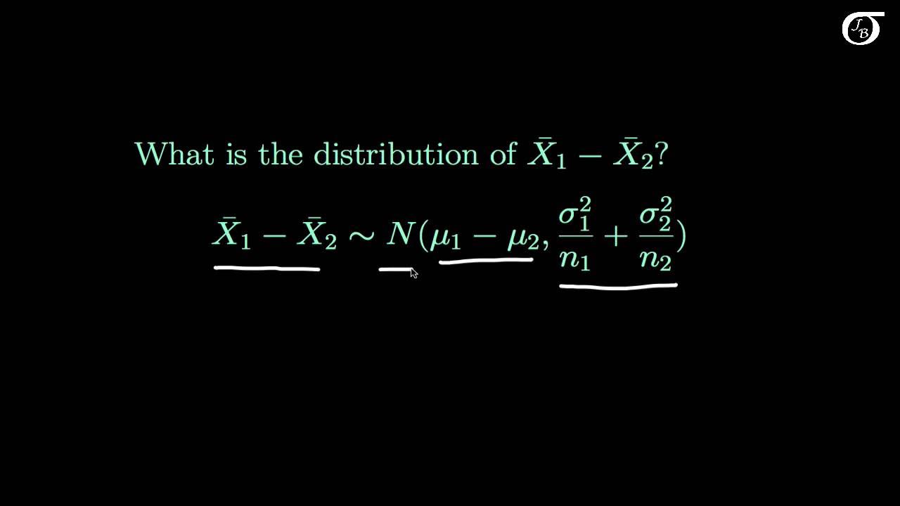
The Sampling Distribution of the Difference in Sample Means (X_1 bar - X_2 bar)

Central Limit Theorem & Sampling Distribution Concepts | Statistics Tutorial | MarinStatsLectures

What is a Sampling Distribution? | Puppet Master of Statistics

Amostras e Erro Amostral Bioestatística #7

Sampling Distributions: Introduction to the Concept
5.0 / 5 (0 votes)
