Kirchhoff's Voltage Law (KVL)
Summary
TLDRIn this lecture, the speaker explains Kirchhoff's Voltage Law (KVL), stating that the algebraic sum of voltages in a closed loop is zero. Using an example circuit with a voltage source and two resistors, the speaker walks through applying KVL to find the voltage drops across each component. They also introduce two different sign conventions for writing KVL equations, discussing the relationship between voltage, current, and resistance. Lastly, the speaker emphasizes the importance of understanding the concept behind KVL, based on energy conservation, to solve circuits effectively.
Takeaways
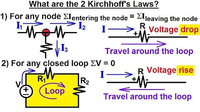
- 📏 The lecture begins with a discussion of KVL (Kirchhoff’s Voltage Law), stating that the algebraic sum of all voltages in a closed loop is zero.
- 🔋 In a closed loop with a voltage source (V), a resistor (R1), and another resistor (R2), the sum of voltage drops equals the total voltage supplied.
- 💡 KVL can be applied by adding up the voltage drops across each element in the loop, where voltage drops across resistors are calculated using Ohm’s law (V = IR).
- 🔄 The potential drop across a resistor is determined by multiplying the current (I) by the resistance (R).
- 🔍 Two conventions for writing KVL equations: the first considers a rise in potential as positive, while the second considers a rise as negative.
- 📝 Both conventions lead to the same result, with V = I * (R1 + R2), showing that the total voltage drop equals the source voltage.
- 🌍 KVL is based on the law of conservation of energy, as opposed to KCL (Kirchhoff's Current Law), which is based on the conservation of charge.
- ⚡ Voltage represents potential energy difference, meaning the energy to move a unit charge between two points is independent of the path taken.
- 🎯 KVL equations should include only potential differences (voltages) between points, not individual point potentials.
- 🔁 The lecture emphasizes that regardless of the chosen path in a circuit, following proper rules will always yield consistent results.
Q & A
What is KVL?
-KVL stands for Kirchhoff's Voltage Law, which states that the algebraic sum of all the voltages in any closed loop of a network is zero.
How do you apply KVL?
-To apply KVL, you calculate the sum of all voltages in a closed loop, considering their signs, and set this sum equal to zero.
What is the significance of the voltage source in the KVL equation?
-The voltage source in the KVL equation is represented by 'V' and is considered as a rise in potential, which is typically given a positive sign in the KVL equation.
What is the role of resistors in the KVL equation?
-Resistors in the KVL equation represent voltage drops across them, calculated as the product of current (I) and resistance (R), and are typically given a negative sign due to the drop in potential.
How does the direction of current flow affect the KVL equation?
-The direction of current flow determines whether the potential rises or drops. A rise in potential is associated with a positive sign, while a drop is associated with a negative sign in the KVL equation.
What are the conventions for writing KVL equations?
-There are two main conventions: one where a rise in potential is positive and a drop is negative, and another where the signs are reversed. The choice of convention depends on the direction chosen to traverse the loop.
Why is KVL based on the law of conservation of energy?
-KVL is based on the law of conservation of energy because voltage represents the potential energy difference across an element, and the energy required to move a unit charge between two points is independent of the path taken.
How do you calculate the potential difference between two points using KVL?
-To calculate the potential difference between two points using KVL, you choose a path between those points, apply KVL up to the second point, and equate the result to the potential at the second point.
Why can't you include the potential at a point directly in the KVL equation?
-You can't include the potential at a point directly in the KVL equation because KVL deals with potential differences (voltages), not absolute potentials.
What happens if you apply KVL starting from different points in the circuit?
-Applying KVL from different starting points should yield the same result for the potential difference between any two points, as long as the rules are followed correctly.
How does the choice of path affect the KVL equation?
-The choice of path affects the order in which voltages are added to the KVL equation, but the final result for the potential difference between any two points should be the same regardless of the path chosen.
Outlines
🔍 Introduction to KVL and Voltage Calculation in a Closed Loop
In this paragraph, the speaker introduces Kirchhoff's Voltage Law (KVL), which states that the algebraic sum of all voltages in a closed loop is zero. The explanation involves a simple circuit with a voltage source and two resistors. The potential difference between points in the circuit is calculated, illustrating the concept of high and low potential, as well as voltage drops across resistors according to Ohm's law. The paragraph ends by formulating a basic KVL equation.
⚖️ Understanding Sign Conventions in KVL
This paragraph focuses on two different conventions for writing KVL equations. The first convention assigns a positive sign to rises in potential and a negative sign to potential drops. An example is given where moving through the circuit components leads to forming the KVL equation. The second convention reverses the sign conventions—assigning a negative sign to potential rises and a positive sign to potential drops. Despite the differences in conventions, the final equation remains consistent. The speaker suggests that the second convention is more intuitive for them.
🔋 KVL and the Conservation of Energy
Here, the relationship between KVL and the law of conservation of energy is explained. KVL is derived from the principle that voltage is a measure of potential energy difference across an element, which remains independent of the path chosen between two points. The speaker provides an example of calculating potential differences between two points, VA and VB, and explains that KVL deals only with voltages or potential differences, not the potentials themselves.
🧠 Applying KVL to Solve Potential Differences
This paragraph provides a method for solving potential differences using KVL. The speaker explains how to start from a point, apply KVL by considering only potential differences (voltage sources and drops across resistors), and avoid using individual potentials at points in the circuit. An example of solving for VA - VB is presented, showing how to follow different paths in the circuit and still arrive at the same result. The speaker emphasizes the importance of understanding concepts over memorizing formulas.
Mindmap
Keywords
💡KVL (Kirchhoff's Voltage Law)
💡Closed loop
💡Voltage drop
💡Ohm's Law
💡Potential difference
💡Resistor
💡Series circuit
💡Conventions for potential rise and drop
💡Law of conservation of energy
💡KCL (Kirchhoff's Current Law)
Highlights
Introduction to KVL (Kirchhoff's Voltage Law)
KVL states the algebraic sum of all voltages in a closed loop is zero
Explanation of how to calculate the sum of voltages considering their signs
Example of a closed loop with a voltage source and two resistors
Concept of potential difference and how it relates to voltage
How to determine the potential at different points in a circuit
Application of Ohm's law to calculate voltage drop across resistors
Derivation of the KVL equation for the example circuit
Introduction to conventions for writing KVL equations
First convention: rise in potential is positive, drop is negative
Second convention: rise in potential is negative, drop is positive
Explanation of why KVL is based on the law of conservation of energy
How voltage is a measure of potential energy difference
The uniqueness of voltage values and their independence of path
How to apply KVL when calculating potential differences between points
Emphasis on not including point potentials in KVL equations
Demonstration of calculating VA - VB using KVL
Explanation of choosing different paths to calculate potential differences
Final statement on the consistency of results when applying KVL correctly
Encouragement to clarify concepts for easy problem-solving
Transcripts
in the last lecture we had discussion on
KCl and now we are going to understand
what is KVL and how to apply KVL so
let's move on to this statement of KVL
the algebraic sum of all the voltages in
any closed loop is zero so when you
calculate there is a break sum of all
the voltages this means you calculate
the sum of all the voltages considering
their signs then you will find it is
equal to zero in closed loop for example
here we have a closed loop having three
elements first one is the voltage source
providing the voltage V second one is a
resistor having the value R one the
third one is resistor again but having
the value R 2 now let's say the current
in this loop is equal to I and we know
the potential difference or the voltage
is equal to the high potential minus the
low potential let's say this point is
connected to the ground this means here
we will have zero volt as the potential
and therefore here also we will have
zero volt as the potential and therefore
this point is still low potential point
and let's say potential here is equal to
V Prime
this is the high potential point so the
high potential that is V Prime minus the
low potential that is zero volt will be
equal to the potential difference or the
voltage which is V therefore we can say
that V prime is equal to V so the
potential here that is V prime is equal
to V now we know the fact that when
current I passes through resistance r1
there will be four
drop and the voltage drop will be equal
to current I multiplied to r1 following
the Ohm's law here potential is V this
means here also potential will be V and
this potential will get reduced by hi I
1 because this is the potential drop due
to resistance r1 so here we will have
the potential equal to V minus I R 1 hi
r1 so here also we will have the
potential equal to V minus hi hi 1 R 1
and R 2 are connected in series
therefore same current I will flow
through r2 as well and therefore the
drop across R 2 will be equal to I
multiplied to r2 therefore when we move
to this point this potential will reduce
by hi r2 so V minus I R 1 minus hi r2
will be the potential at this point but
this point is having the potential equal
to zero volt this implies V minus I R 1
minus IR to V minus I R 1 minus I R 2 is
equal to zero and this is our KVL
equation so I hope you now understand
how to find the KVL equation but every
time we are not going to analyze this
circuit like this there are some
conventions and following those
conventions you can write down the KVL
equation directly and there are
different ways to write down the KVL
equation here we have followed the
convention in which we are considering
the rise in potential as positive I will
first write down the convention and then
we will follow it in this particular
Rickett so the convention is rise in
potential will give you the positive
sign and the drop in potential who will
give you the negative sign now focus on
this particular voltage source we are
starting from this point and then we
will move back to this point and the
first element we are encountering is a
voltage source now when you move from
this point to the upward direction you
can see that we first encountered the
negative terminal this means the low
potential point and then we encountered
the positive terminal
this means the high potential point so
low to high
this means rising potential and
therefore we will have the positive sign
for V so we will write plus V then we
will keep on moving and we encountered a
resistance r1 so here we are having the
voltage drop by I R 1 and we know
resistor will dissipate the power and
therefore current will enter the
positive terminal and it will leave the
negative terminal we have already
discussed at this point in great detail
so here you can see that we first
encountered the high potential point and
then we encountered the low potential
point so there is drop in potential
hence we will have the negative sign so
negative I r1
I R 1 similarly here also we will have
the drop in potential therefore we will
write minus hi r2 and this will be equal
to 0
so you can see that we have the same
equation and from here we can say that V
is equal to AI
r1 plus r2 now I will give you the
second convention and according to this
convention the rise in potential will
give you the negative sign opposite of
this convention and the drop in
potential who will give you the positive
sign this convention is reversed here
and now we will obtain the KVL equation
following the new convention we will
start from this point and we will
encounter an element that is the voltage
source and you can see that we are
having the rise in potential therefore
we will have the negative sign so minus
V then we encounter another element that
is a resistor and here we are having the
fall or drop in potential therefore we
will have the positive sign and then we
have I R 1 i R 1 similarly we have plus
I R 2 for resistor r2 plus hi r2 and the
sum we are going to get is equal to 0
and from this equation we can say that
voltage V is equal to I multiplied to r1
plus r2 the same result now please let
me know in the comment section which
convention do you want to follow I
personally like to follow this
convention because this makes more sense
to me now
we will move on to the last point and
according to this point
KVL his based on law of conservation of
energy
KCl was based on law of conservation of
charge but KVL is based on law of
conservation of energy the voltage is
the measure of potential energy
difference across the element we know
this point
and we also know that there is a single
unique value of a voltage therefore the
energy required to move a unit charge
from one point to other his independent
of the path chosen you will get the same
voltage or potential difference between
the two points irrespective of the path
you have chosen for example let's say
this point his point a and this point
his point B and potential here is equal
to VA and potential here is equal to VB
and we want to calculate the potential
difference VA minus VB that is we want
to calculate the difference in the
potentials of the point a and the point
B we want to have the potential
difference VA minus VB and due to our
initial analysis we know the potential
at Point a is equal to zero volt and the
potential at point B is equal to V minus
I R 1 so we can write VA minus VB equal
to 0 minus V minus I R 1 or we can write
minus V plus I R 1 so this is the
potential difference VA minus VB the
potential difference between the point a
and the point B but every time you won't
have the potentials at the two points
and therefore you must know how to apply
KVL when you are required to calculate
the potential difference between the two
random points in the circuit and we know
KVL is the voltage law voltage means the
potential difference and therefore in
the KVL equation you will only have the
voltage or potential difference all the
three values here our voltages V is the
voltage hi r1 is
I r2 is also a voltage so you cannot
include the potential at a point in KVL
equation this means you cannot include
VA and you cannot include VB but you can
include VA minus VB because VA minus VB
is the potential difference or the
voltage so I will now explain how to
deal with this kind of problem whenever
you have to deal with the potentials at
a point then pick one point for example
pique then write down the potential at
ay that is VA I will write here then
simply apply KVL up to this particular
point move in this direction you will
have a voltage source V following this
convention we will write plus V Plus V
then we will move forward and have one
resistance therefore we will have minus
hi hi 1 now when you move at this point
then don't write VB like this and equate
it with zero you have to write equal to
and then instead of equating with zero
equate it with V B now in this scenario
when you subtract V B from both the
sides you have VA minus VB plus V minus
y1 equal to zero now this is proper KVL
equation this is one very powerful way
and we will use it a lot to solve the
questions in this course so from here we
will have VA minus VB equal to minus V
Plus hi hi 1 the same result there is
one point I want to clear you can see
that while applying the KVL starting
from the point a we did not included the
potential here which
we so whenever you apply kvl from one
point to another point don't include the
other potentials at point because your
KVL will then be in valid so simply
start with potential at a point and then
include only potential differences and
then finally equate everything with the
final points potential so I hope this
was clear now we have chosen one path to
calculate VA minus VB we can choose
another path as well
so now let's calculate VA minus VB
following this path we will start from
point A and we will have VA then we will
have plus I R 2 plus i r2 and then we
will stop at point B therefore we will
equate with potential VB from here we
are getting VA minus V B equal to minus
hi r2 and VA minus VB we have calculated
should be equal therefore minus V plus I
R 1 should be equal to minus I R 2 this
implies we will have minus V plus I R 1
equal to minus I R 2 and from here we
can say that V is equal to Y R 1 plus R
2 the same result so whatever you do in
the circuit following the proper rules
you will finally have the same result
you don't have to mug up anything you
simply have to clear your concepts and
if your concepts are clear you can
easily solve any network so I hope this
lecture was clear to you and if you have
any doubt you may ask in the comment
section I will hand this lecture here
see you in the next one
[Applause]
you
[Music]
Ver Más Videos Relacionados
Kirchhoff's voltage law | Circuit analysis | Electrical engineering | Khan Academy
HUKUM II KIRCHHOFF
Chapter 2 - Fundamentals of Electric Circuits
thevenin's theorem explanation | Thevenin's Theorem Solved Example Problem
Load Line Analysis of Diode
DC Series circuits explained - The basics working principle
5.0 / 5 (0 votes)