The Discrete Fourier Transform (DFT)

Summary

This video introduces the Discrete Fourier Transform (DFT), explaining its role in converting discrete data into Fourier coefficients to analyze signals. The speaker clarifies how DFT differs from the continuous Fourier Transform and emphasizes the importance of the Fast Fourier Transform (FFT), a highly efficient algorithm widely used in fields like audio compression, image processing, and scientific computing. The mathematical concepts behind DFT are explored, with the speaker highlighting how it can be written as a matrix multiplication and how FFT enables faster computation of large datasets.

Takeaways

• 🧮 The Discrete Fourier Transform (DFT) is key for computing Fourier series on discrete data.
• 📉 DFT approximates a Fourier series for a finite, periodic interval of data rather than an infinite Fourier transform integral.
• 🖥️ The Fast Fourier Transform (FFT) is a computationally efficient way to compute the DFT, especially for large datasets.
• 🎶 DFT is used to decompose data into sine and cosine components, which is valuable for tasks like signal processing and diagnostics.
• 🔢 Input data for DFT is represented as a vector of discrete values, which may be sampled from continuous functions.
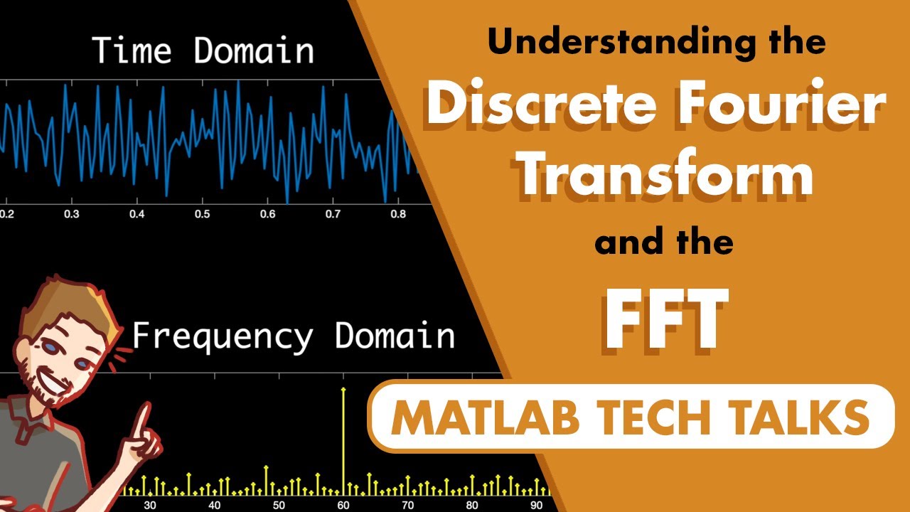
• 📊 DFT transforms this discrete data into Fourier coefficients, revealing the frequencies present in the data.
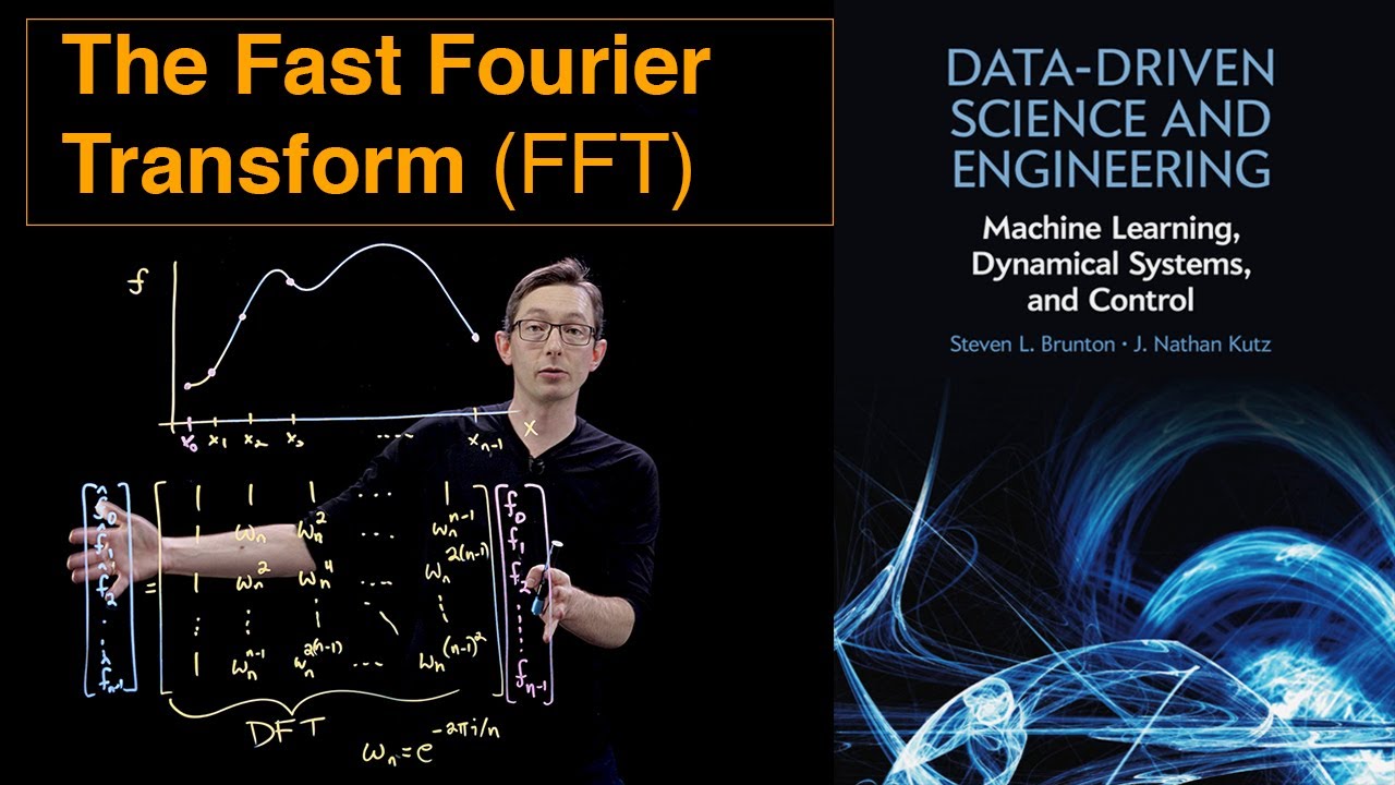
• 🧩 The transformation process involves a matrix multiplication, where the DFT is defined mathematically using exponential terms.
• 🔄 You can also reconstruct the original data from the Fourier coefficients using an inverse DFT formula.
• ⚙️ The FFT allows efficient computation of the DFT without explicitly performing large matrix operations.
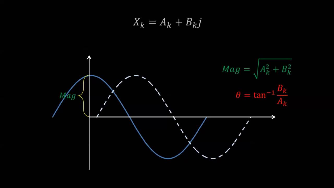
• 🌀 The result of the DFT includes complex numbers, with the magnitude indicating the frequency's strength and the phase indicating its alignment.

Q & A

What is the Discrete Fourier Transform (DFT)?

The Discrete Fourier Transform (DFT) is a mathematical transformation that approximates a Fourier series on a finite interval where the function is periodic. It allows one to convert data points from the time domain into frequency components, revealing the sine and cosine components that make up the signal.

Why is the name 'Discrete Fourier Transform' considered misleading?

The name 'Discrete Fourier Transform' is considered misleading because it more accurately represents a Fourier series approximation rather than a true Fourier transform, which involves an integral over infinite intervals. However, due to historical reasons, it is called DFT.

What is the relationship between the DFT and the Fast Fourier Transform (FFT)?

The FFT is a computationally efficient algorithm to compute the DFT. While the DFT can be calculated through direct matrix multiplication, the FFT reduces the computation time significantly, making it feasible to process large datasets.

What are some applications of the Fast Fourier Transform (FFT)?

The FFT is widely used in areas such as image compression, audio compression, signal processing, and high-performance scientific computing. It's considered one of the most powerful and important algorithms of the 20th century.

What is the basic idea behind using Fourier series to approximate functions?

Fourier series approximates a function by breaking it down into a sum of sine and cosine terms. This is particularly useful for periodic functions, where the series captures the frequency components that make up the signal.

How is the DFT applied to experimental or simulation data?

The DFT is applied to discrete data points obtained from experiments or simulations, assuming an underlying continuous function. The DFT converts these discrete data points into frequency components that describe the signal.

What is the mathematical representation of the DFT?

The DFT of a dataset is represented as a sum over data points, where each data point is multiplied by a complex exponential term. This sum results in a set of Fourier coefficients, representing different frequency components in the data.

What is the inverse DFT, and how does it work?

The inverse DFT allows one to reconstruct the original data from its Fourier coefficients. It involves summing over the frequency components, using a similar formula to the DFT but with a positive exponential term and a normalization factor of 1/N.

What is the significance of the complex exponential terms in the DFT?

The complex exponential terms in the DFT represent the sine and cosine components of different frequencies. They allow the transformation of time-domain data into frequency-domain data by capturing both the magnitude and phase of each frequency component.

How is the DFT represented as a matrix operation?

The DFT can be written as a matrix operation, where the data vector is multiplied by a matrix of complex exponential terms (DFT matrix) to obtain the Fourier coefficients. This matrix approach simplifies the computation, especially for large datasets.

Why is the FFT preferred over directly computing the DFT?

The FFT is preferred because it provides a highly efficient way to compute the DFT without constructing and multiplying large matrices. The FFT significantly reduces the computation time, making it practical for real-time applications and large datasets.

Outlines

00:00

📊 Introduction to Discrete Fourier Transform (DFT)

The speaker begins by discussing the Fourier series and Fourier transforms, emphasizing the importance of the Discrete Fourier Transform (DFT) in computing. They humorously suggest that DFT should be named the Discrete Fourier Series because it approximates the Fourier series on a finite interval. The DFT is crucial for applications like image and audio compression, signal processing, and scientific computing. The Fast Fourier Transform (FFT), an efficient algorithm for computing the DFT, is highlighted as one of the most significant algorithms of all time. The lecture aims to explain the DFT in terms of matrix multiplication and its application in transforming data vectors into their sine and cosine components, which can be useful for various applications, including diagnosing car issues through audio signal analysis.

05:01

🔍 Computing Fourier Coefficients

The speaker explains the process of computing Fourier coefficients from data points. They describe how to transform a data vector into its frequency components using the DFT. The Fourier coefficients are obtained by summing over all data points, multiplied by a complex exponential term. The inverse DFT is also discussed, which allows reconstruction of the original data from its Fourier coefficients. The concept of a fundamental frequency, denoted as Omega_n, is introduced as a key element in the computation of the DFT matrix. The speaker clarifies that the Fourier transform and its inverse involve complex exponentials with positive and negative exponents, respectively, and both are normalized differently.

10:03

🧮 Matrix Representation of DFT

The speaker illustrates how the DFT can be represented as a matrix operation, where the data vector is multiplied by the DFT matrix to obtain the Fourier transform vector. They discuss the tediousness of computing the DFT using a direct summation approach and instead propose a matrix representation that simplifies the computation. The matrix is constructed using the fundamental frequency Omega_n, and the speaker provides an example of how the matrix looks for different values of K. The first row of the matrix is all ones, representing the constant value or zeroth frequency, while subsequent rows represent higher frequencies. The speaker emphasizes that the DFT matrix is complex and that each entry in the Fourier coefficients vector is a complex number, indicating both the magnitude and phase of the corresponding frequency component.

15:03

🚀 Efficiency through Fast Fourier Transform (FFT)

The speaker concludes by acknowledging the computational expense of directly computing the DFT using the matrix approach. They hint at the upcoming discussion on the Fast Fourier Transform (FFT), an algorithm that efficiently computes the DFT without constructing the entire matrix. The FFT is a crucial tool for handling large datasets and is fundamental to many modern computational applications. The speaker assures that the mathematical definition of the DFT will be practically applied through the FFT in subsequent lectures.

Keywords

💡Fourier Transform

A mathematical technique used to transform a function into its frequency components. In the context of the video, it's applied to understand the breakdown of complex signals (like audio or data) into simpler sine and cosine waves. The Fourier Transform allows one to analyze the frequency content of signals.

💡Discrete Fourier Transform (DFT)

The DFT is a computational method used to analyze discrete data points, as opposed to continuous signals, by transforming them into frequency components. The video emphasizes that while the term might be misleading, the DFT is more akin to a Fourier series approximation over a finite interval of data.

💡Fast Fourier Transform (FFT)

A highly efficient algorithm used to compute the DFT in a computationally fast manner, which is essential for processing large datasets. The video highlights the FFT as one of the most important algorithms in modern computation, essential for applications such as image and audio compression.

💡Fourier Series

A mathematical representation of periodic functions as an infinite sum of sine and cosine terms. In the video, it's used to introduce the concept of approximating complex data sets by breaking them into simple periodic functions, especially when working with data from simulations or experiments.

💡Data Vector

A collection of discrete data points representing a function in a numerical or experimental setting. The video uses the example of experimental measurements or simulation outputs as vectors of data that can be transformed via DFT to extract frequency components.

💡Frequency Components

These are the individual sine and cosine waves that combine to form a complex signal or function. In the video, the speaker explains that the DFT breaks down the data vector into its frequency components, revealing how much of each frequency contributes to the overall signal.

💡Fourier Coefficients

The weights or amplitudes of the sine and cosine functions in the Fourier series. In the video, the Fourier coefficients (denoted as f1 hat, f2 hat, etc.) are explained as the key output of the DFT, representing how much of each frequency is present in the data.

💡Matrix Multiplication

A mathematical operation that applies to arrays of numbers, used to represent the DFT in the video. The speaker describes how the DFT can be written as a large matrix multiplication that transforms a data vector into its corresponding Fourier coefficients.

💡Exponential Function

A mathematical function of the form e^(ix), where i is the imaginary unit and x is a real number. This function plays a central role in the DFT, as it appears in the summation formula to calculate the Fourier coefficients. The video explains the complex nature of this function and its significance in frequency decomposition.

💡Phase and Magnitude

The phase indicates the shift of a sine wave, while the magnitude represents the amplitude. In the video, the Fourier coefficients are described as complex numbers whose magnitude gives the strength of a frequency component, while the phase determines the wave's alignment (sine or cosine).

Highlights

Introduction to the Discrete Fourier Transform (DFT) and its significance in computing.

The DFT is often misnamed and should be called the Discrete Fourier Series.

Explanation of the DFT as an approximation of the Fourier series on a finite interval.

The importance of the Fast Fourier Transform (FFT) as a powerful algorithm.

Applications of the FFT in various fields like image and audio compression, signal processing, and scientific computing.

The mathematical transformation of the DFT can be represented as a matrix multiplication.

The FFT provides a computationally efficient way to compute the DFT for large datasets.

The process of approximating periodic functions using sums of sines and cosines.

The common scenario of having discrete data points rather than an analytic function.

The concept of transforming a data vector into its sine and cosine components through DFT.

Practical use case: Diagnosing car issues through audio signal analysis using DFT.

The DFT can also be used to compute or approximate derivatives of data.

Explanation of the formula for computing the DFT and obtaining Fourier coefficients.

The inverse DFT formula for reconstructing data from Fourier coefficients.

The significance of the fundamental frequency in the context of DFT.

The DFT matrix and how it can be used to transform data into Fourier coefficients.

The complex nature of Fourier coefficients and their interpretation in terms of magnitude and phase.

The computational expense of directly computing the DFT matrix and the need for the FFT.

Upcoming lectures will cover the efficient computation of the DFT using the FFT.

Transcripts

[Music]

welcome back so we're talking about the

Fourier series Fourier transforms and

now I'm going to tell you about how you

compute these in a computer using the

discrete Fourier transform okay so this

is really really important the discrete

fourier transform and I think this is

actually I always joke with my students

that this is kind of a terrible name

really this should be called a discrete

Fourier series because what we're

actually doing is we're approximating

that Fourier series approximation on a

finite interval where your function is

periodic that's what we're actually

approximating is the finite series and

not the infinite Fourier transform

integral but through some joke of

history it is now called the discrete

Fourier transform or the DFT and this is

an extremely important concept which

will eventually lead to the fast Fourier

transform the FFT which is probably the

most powerful algorithm of the last

century maybe of all time it's one of

the most important algorithms today it's

used for image compression audio

compression signal processing

high-performance scientific computing

you name it fast Fourier transform is

probably at the heart of some of these

computations and what I want to get

across right now is that the discrete

Fourier transform is a mathematical

transformation that can be written in

terms of a big matrix multiplication the

fast Fourier transform is a

computationally efficient way of

computing the DFT

that scales to very very large datasets

so in some sense these are kind of

synonymous the FFT is how we compute the

DFT okay but today I'm going to tell you

about the DFT the discrete Fourier

transform and soon I'll show you how to

actually can numerically implement this

via the FFT okay so we talked about

approximating functions that are

periodic using infinite sums of sines

and cosines let me show that this is

this is possible but in many many cases

most of the time I don't

have an analytic function I have

measurement data from an experiment or

from a simulation okay so what I what I

often have is some F defined at discrete

locations x1 x2 x3 all the way up to

some X n so I have a discrete vector of

data some function and maybe we believe

that there's a continuous function

underlying this data but I'm only

sampling it at these discrete locations

x1 and x2 x3 and so on and so forth up

to X n okay so what I have is a vector

of data in fact I'm just gonna literally

write this out I have a vector of data

f1 f2 f3 dot dot dot all the way down to

F and okay this is gonna be my I'm just

gonna call this you know some some

vector of data and what I'm gonna want

to do is Fourier transform compute the

discrete Fourier series of that data

vector okay so I also want to break this

data up into a sum of sines and cosines

and this can be very useful you can

figure out if this is audio data you can

figure out what are kind of the the

tones that add up to make that audio

data I always tell my students you know

what I want to do is build an iPhone app

so you put it on the roof of your car or

the hood of your car and it listens to

the audio signal it computes the Fourier

transform and based on the frequency

content maybe it can diagnose if

something's wrong with your car like you

have a belt slipping or some kind of

vibration that shouldn't be there okay

so so turning a data vector into its

sine and cosine components through this

discrete Fourier transform can be very

very useful it's also nice to compute

derivatives to approximate derivatives

of of data using using these Fourier

transform derivative properties okay so

I'm gonna walk you through what the

Fourier transform the discrete Fourier

transform is how you can write it as a

big matrix multiplication but remember

it's basically just a Fourier series on

data

instead of on contingent on functions

analytic functions okay so let's just

get started so I'm just gonna write down

what the the 48 discrete Fourier

transform is and then I'm going to show

you some ways of interpreting this okay

so for each of these data points FK what

we're going to be able to do is compute

a as you might imagine what we're going

to try to get out of this is some vector

of Fourier coefficients f1 hat f2 hat f3

hats all the way down to F and hat so

just like we took our function f and we

turned it into these coefficients that

multiplied our cosine and sines that's

what we're doing here we're taking our

data F and we're going to obtain this

Fourier transform vector F hat of

frequency components so f1 hat will tell

me how much of that first low frequency

is in the data f2 hat will tell me how

much of that next higher frequency is in

the data and so on and so forth where FN

hat is the highest frequency possible

with n data points if it was going you

know as fast as possible oscillating

over n data points and so the way that

we get that F hat vector we say that F

hat K maybe I'll write it up here F hat

K the caithe Fourier coefficient is a

sum over all of my all of my data to n

minus 1 of my data F J the J element of

my data times e to the minus I 2 pi J K

over N this is kind of a pain I'll walk

you through all of these terms here ok

so the case Fourier coefficient is

obtained by taking the sum over all J

data points at the jet frequency times

the caithe frequency divided by N and

I'll tell you what this kind of e to the

I 2 pi JK over n means in a minute ok

but this is how you compute all of those

case Fourier coefficients and similarly

just like an ax for you

transform or a Fourier series if I have

my data I can get my Fourier transform

but if I have my Fourier transform I

should be able to go back and

reconstruct my data it's all write down

what that is and it's again it's pretty

similar so FK once I had all of these

blue hats the FK is again a sum over all

frequencies now of J equals 0 to n minus

1 of my F J hat ok my J Fourier

coefficient times now e to the positive

I 2 pi JK over N so this is very very

similar to the Fourier transform pair

where this is a negative exponent and

this is a positive exponent and this

whole thing is times 1 over N remember

just like in the Fourier transform this

had a 1 over I think pi or 2 pi this

also has to a slightly different

normalization ok and so what this means

is that if I have if I have my data kind

of F 1 F 2 dot dot

to F n I can run it through this Fourier

transform this DFT this discrete Fourier

transform here this is my DFT and I can

get my Fourier frequencies f1 hat f2 hat

dot dot F and hat ok and these literally

are the f1 f2 F and hats are literally

telling me how much of each each

frequency I need to add up to

reconstruct this data in in F ok and

there will be some subtleties I'll tell

you about but to compute this thing this

is kind of interesting is that notice

that all of these these these terms in

this series are multiplying these

Exponential's which are some integer

multiple of e to the I to PI over N ok

so we have this kind of e to the minus 2

pi I over N I is the the complex the

imaginary

i square root of one I'll just write I

equals square root of negative one okay

this is I and this defines a fundamental

frequency that's defined some Omega n

okay which is some fundamental frequency

that is related to two what kinds of

sines and cosines I can approximate with

n discreet values in a domain X okay so

this is kind of the fundamental

frequency we get to work with if I have

an interval with n data points and all

of these Fourier transforms are adding

up integer multiples of that fundamental

frequency times my data and the same

thing with my inverse Fourier transform

okay so we're gonna be able to use this

fundamental frequency Omega n to compute

a matrix that would multiply my data and

give me my Fourier transform so that's

really really important and I'm gonna

write this out here okay okay good so so

we have this this sum over the data to

compute the Fourier transform and the

inverse Fourier transform but I don't

want to go you know for K 1 for K 2 for

K 3 4 K 4 and compute this whole sum

this seems very tedious this would be

kind of too big for loops if I wanted to

actually code that up and I don't want

to do that so instead what we're going

to do is we're going to try to write

what this sum would be for each of these

k's in terms of a matrix operation where

i take my data vector and i multiply it

by a matrix to get my Fourier transform

vector and I'm gonna write it in terms

of these fundamental frequencies Omega

ends okay and I'll point out you can

absolutely go back to your definition of

the Fourier series the complex Fourier

series where you had it written in terms

of the complex exponential and you can

show that this is exactly what you would

get if you took your your Fourier series

and approximated it with N and discrete

values in the middle this is exactly

analogous to the cosines and sines of

those discrete frequencies in the

Fourier series okay good so we have this

fundamental frequency and we're going to

walk through and sometimes what I like

to do is just think if K

was one what would this series look like

okay so if K was one I would take all of

my f J's and multiply them by some the

first row vector and that would tell me

the coefficient on each of those f JS

okay now if K was yeah I probably should

have k zero yeah sorry I'm being pretty

sloppy here let's say that I actually

have a 0th index here let's say I have

an x0

and that this is f0 f1 f2 all the way up

to FN and this is f0 f1 f2 all the way

up to FN this will make a lot more sense

if J my data has to be indexed from 0 to

n minus 1 okay so the 0th this is the

0th frequency kind of the constant value

if I had K equals 0 here then all of my

exponents would be e to the I times 0

because K is 0 and e to the 0 is 1 no

matter what J is if K is 0 this whole

exponent is 1 is that is this whole

exponent is 0 so e to the 0 is 1 and so

the coefficient on every single data

point here is 1 and I'm adding up F 0

plus F 1 plus F 2 plus F 3 all the way

to F n that will give me the first the

zeroth F hat so this row is 1 maybe I'll

make it in yellow this is is 1 1 1 dot

dot dot 1 okay this entire first row is

just ones now for the second row now

let's figure out what happens for F 1

hat okay so in K equals 1 now all of

these coefficients multiplying my data F

for J equals 0 I get e to the 0 is 1 ok

for J equals 1 I get e to the minus 2 pi

divided by n remember K is 1 so that's

just Omega when J equals 2 I get

basically Omega squared I get e to the

minus 2 pi I times 2 divided by n this

is Omega N squared

dot dot dot and eventually at the very

end I'll have Omega n to the power n

minus 1 ok and I can keep going down if

K was 2 then I would have everything you

know multiplying 2 in the exponent so I

would still have for J equals 0 a 1 here

I would have an Omega N squared because

my K is 2 I'd have Omega N to the 4th

dot dot dot Omega and to the 2 n minus 1

and so on and so forth you can just go

down the list I'll always have ones on

the first row and the first column down

here I'm gonna have something like Omega

N to the N minus 1 Omega n to the 2 n

minus 1 dot dot dot and eventually this

last entry is going to be Omega n to the

N minus 1 squared ok so this is

something you can you can readily kind

of convince yourself that every row of

this is one value of K here and you can

figure out what the coefficients are of

the data that will be the row of this

matrix DFT here okay so long story short

what I'm trying to convince you of is

that if you have a data vector instead

of an analytic function so you just have

data in these these pink dots here you

can still compute something like a

fourier series like a fourier transform

but it's the discrete Fourier transform

okay and the form of the the discrete

Fourier transform pair to go from data

to Fourier coefficients or to go from

Fourier coefficients back to your data

looks very much like a Fourier series

but because this is defined on discrete

data I can write it as a big matrix

operation okay so this here is the DFT

matrix this is the DFT the discrete

Fourier transform matrix and if you had

your your vector of data you multiply it

by this matrix you get your Fourier

transform out very very useful okay and

these Fourier coefficients you'll notice

that this is a complex number okay this

is e to the this has a cosine plus an I

sine part this is a complex number so

this is a complex matrix and these

Fourier coefficients these blue Fourier

coefficients are complex valued and so

these somehow tell you how much of that

0th mode cosine and sine mode there are

but it also tells you the phase okay so

the magnitude of this complex number

tells you how much magnitude of that

first mode you have and then the cut the

the phase angle of that complex number

tells you you know how much cosine or

how much sine or what phase in between

your your sine and cosine is okay so

every single one of these values is a

complex number and the magnitude tells

you how much of that set that that

second frequency sine and cosine you

have and the phase tells you what is the

the phase between cosine and sine and it

gives you exactly the sines and cosines

you need to add up to approximate your

data perfectly okay so this is the

discrete Fourier transform this is

pretty expensive to actually compute

this matrix and multiply your data to

compute this Fourier transform and so

what I'm going to show you in the next

few lectures is how you compute this

efficiently using the fast Fourier

transform so you never actually have to

build this matrix and do this

multiplication this is how its

mathematically defined but

computationally we're always going to

compute the DFT

using the fast Fourier transform

algorithm okay that's all coming up soon

thank you