Perceptron Training

Udacity
23 Feb 201509:25

Summary

TLDRThis script delves into machine learning's weight determination, focusing on the Perceptron Rule and gradient descent. It simplifies the learning process by treating the threshold as a weight, allowing for easier weight adjustments. The Perceptron Rule is particularly highlighted for its ability to find a solution for linearly separable data sets in a finite number of iterations. The discussion touches on the algorithm's simplicity and effectiveness, and the potential challenge of determining linear separability in higher dimensions.

Takeaways

  • 😀 The script discusses the need for machine learning systems to automatically find weights that map inputs to outputs, rather than setting them by hand.
  • 🔍 Two rules are introduced for determining weights from training examples: the Perceptron Rule and the Delta Rule (gradient descent).
  • 🧠 The Perceptron Rule uses threshold outputs, while the Delta Rule uses unthreshold values, indicating different approaches to learning.
  • 🔄 The script explains the Perceptron Rule for setting weights of a single unit to match a training set, emphasizing iterative weight modification.
  • 📉 A learning rate is introduced for adjusting weights, with a special mention of learning the threshold (Theta) by treating it as another weight.
  • 🔄 The concept of a 'bias unit' is introduced to simplify the handling of the threshold in weight updates.
  • 📊 The script outlines the process of updating weights based on the difference between the target output and the network's current output.
  • 🚫 It is highlighted that if the output is correct, there will be no change to the weights, but if incorrect, the weights will be adjusted in the direction needed to reduce error.
  • 📉 The Perceptron Rule is particularly effective for linearly separable data sets, where it can find a separating hyperplane in a finite number of iterations.
  • ⏱ The script touches on the challenge of determining when to stop the algorithm if the data set is not linearly separable, hinting at the complexity of this decision.

Q & A

  • What are the two rules mentioned for setting the weights in machine learning?

    -The two rules mentioned for setting the weights in machine learning are the Perceptron Rule and gradient descent or the Delta Rule.

  • How does the Perceptron Rule differ from gradient descent?

    -The Perceptron Rule uses threshold outputs, while gradient descent uses unthreshold values.

  • What is the purpose of the bias unit in the context of the Perceptron Rule?

    -The bias unit simplifies the learning process by allowing the threshold to be treated as another weight, effectively turning the comparison to zero instead of a specific threshold value.

  • How does the weight update work in the Perceptron Rule?

    -The weight update in the Perceptron Rule is based on the difference between the target output and the network's current output. If the output is incorrect, the weights are adjusted in the direction that would reduce the error.

  • What is the role of the learning rate in the Perceptron Rule?

    -The learning rate in the Perceptron Rule controls the size of the step taken in the direction of reducing the error, preventing overshoot and ensuring gradual convergence.

  • What does it mean for a dataset to be linearly separable?

    -A dataset is considered linearly separable if there exists a hyperplane that can perfectly separate the positive and negative examples.

  • How does the Perceptron Rule handle linearly separable data?

    -If the data is linearly separable, the Perceptron Rule will find a set of weights that correctly classify all examples in a finite number of iterations.

  • What happens if the data is not linearly separable?

    -If the data is not linearly separable, the Perceptron Rule will not converge to a solution, and the algorithm will continue to iterate without finding a set of weights that can separate the data.

  • How can you determine if the data is linearly separable using the Perceptron Rule?

    -You can determine if the data is linearly separable by running the Perceptron Rule and checking if it ever stops. If it stops, the data is linearly separable; if it does not stop, it is not.

  • What is the significance of the halting problem in the context of the Perceptron Rule?

    -The halting problem refers to the challenge of determining whether a program will finish running or continue to run forever. In the context of the Perceptron Rule, solving the halting problem would allow us to know when to stop the algorithm and declare the data set not linearly separable.

Outlines

00:00

🤖 Introduction to Machine Learning Weight Setting

The paragraph introduces the concept of setting machine learning model weights automatically through training examples, rather than manually. It contrasts two methods for determining weights: the Perceptron Rule and the Delta Rule (gradient descent). The Perceptron Rule uses threshold outputs, while the Delta Rule uses unthreshold values. The focus then shifts to the Perceptron Rule for setting the weights of a single unit to match a training set. The training set consists of input vectors (x) and desired output values (y). The process involves iteratively modifying the weights to capture the training data. A learning rate for the weights is mentioned, and a trick to learn the threshold (Theta) by treating it as another weight is discussed. This simplifies the process by allowing the threshold to be treated like a weight, eliminating the need to compare against a separate threshold value.

05:03

📊 The Perceptron Learning Rule and Linear Separability

This paragraph delves into the Perceptron Learning Rule, explaining how it updates weights based on the difference between the target output and the network's current output. The weight update is influenced by the learning rate and the input value, ensuring that the model doesn't overshoot the correct solution. The discussion then moves to the concept of linear separability, where if a dataset can be split into positive and negative examples by a line, the Perceptron Rule can find such a line in a finite number of iterations. The paragraph also touches on the challenges of determining linear separability in higher dimensions and the practical approach of running the Perceptron algorithm to see if it converges, which would indicate linear separability. The conversation highlights the theoretical connection between the halting problem and the ability to determine linear separability, suggesting that while solving one might imply solving the other, the converse is not necessarily true.

Mindmap

Keywords

💡Perceptron Rule

The Perceptron Rule is a fundamental concept in machine learning, particularly in the context of supervised learning. It is an algorithm used for training a linear binary classifier. In the video, the Perceptron Rule is discussed as a method for adjusting weights in a neural network to correctly classify a training set, where the output is either 0 or 1. The rule is used to update the weights based on the difference between the predicted output (y hat) and the actual output (y), adjusting the weights to minimize this difference over time.

💡Gradient Descent

Gradient Descent, also known as the Delta Rule, is an optimization algorithm used to minimize a function by iteratively moving in the direction of the steepest descent as defined by the negative of the gradient. In the video, it is mentioned as an alternative to the Perceptron Rule, where it would be used to update weights in a way that considers the unthreshold values of the output, as opposed to the threshold outputs used in the Perceptron Rule.

💡Weights

In the context of the video, 'weights' refer to the parameters of a perceptron (or any neural network) that are adjusted during the learning process. The weights determine the strength and direction of the connections between input neurons and the output neuron. The video discusses how the Perceptron Rule is used to set these weights to map inputs to desired outputs, with the goal of correctly classifying the training data.

💡Threshold

The 'threshold' in a perceptron is a value that the weighted sum of inputs must exceed for the perceptron to output a 1; otherwise, it outputs 0. The video explains a trick to treat the threshold as another weight by adding a bias unit to the inputs, which simplifies the learning process by allowing all comparisons to be made against zero.

💡Bias Unit

A 'bias unit' is an additional input that is always set to 1, and its corresponding weight is used to account for the threshold in a perceptron. By including a bias unit, the threshold can be treated as a weight, which simplifies the learning process. The video script mentions adding a bias unit to the inputs to facilitate learning the threshold as if it were another weight.

💡Learning Rate

The 'learning rate' is a hyperparameter that controls the step size at each iteration while moving toward a minimum of a loss function. In the video, the learning rate is used to scale the weight updates during the training process, ensuring that the updates are not too large, which could cause the algorithm to overshoot the optimal weights.

💡Training Set

A 'training set' is a collection of input-output pairs used to train a machine learning model. In the video, the training set consists of examples with inputs (x) and desired outputs (y), which are used to adjust the weights of the perceptron so that it can correctly classify new, unseen data.

💡Linearly Separable

Data is considered 'linearly separable' if there exists a hyperplane that can separate the data into different classes. The video discusses the Perceptron Rule's ability to find such a hyperplane if the data is linearly separable, which is a key property that allows the perceptron to successfully classify the data.

💡Approximate Output (y hat)

The 'approximate output' or 'y hat' is the predicted output of the perceptron for a given input, before it is thresholded to produce a final classification. In the video, y hat is calculated by summing the inputs according to the current weights and comparing it to zero, which is then compared to the actual output (y) to determine the error and adjust the weights accordingly.

💡Error

In the context of the video, 'error' refers to the difference between the predicted output (y hat) and the actual output (y). The Perceptron Rule uses this error to update the weights, with the goal of reducing the error over the course of training. The video script mentions that if the perceptron correctly classifies the data, the error will be zero, and the weights will not change.

Highlights

The Perceptron Rule and gradient descent are two methods for setting weights in machine learning.

The Perceptron Rule uses threshold outputs, while gradient descent uses unthreshold values.

The Perceptron Rule is used to set the weights of a single unit to match a training set.

A training set consists of input vectors (x) and desired output values (y).

Weights are modified over time to capture the training data set.

A learning rate is introduced for the weights, but a learning rule is given for Theta.

Theta is treated as another weight by adding a bias unit to the inputs.

The threshold can be treated the same as the weights by this method.

The weight change is defined as the difference between the target output and the network's current output.

The weight update is scaled by the learning rate and the input to the unit.

If the output is correct, there will be no change to the weights.

If the output is incorrect, the weights are adjusted to correct the error.

The learning rate controls the magnitude of the weight adjustments to avoid overshooting.

The Perceptron Rule can find a separating line for linearly separable data sets.

The algorithm will stop if a separating line is found, indicating linear separability.

If the algorithm does not stop, it suggests the data may not be linearly separable.

The algorithm's ability to stop can be used as a test for linear separability.

The simplicity of the Perceptron Rule makes it a powerful tool for machine learning.

Transcripts

play00:00

Alright. So in the examples up to this point, we've be

play00:03

setting the weights by hand to make various functions happen. And that's

play00:07

not really that useful in the context of machine learning. We'd really

play00:10

like a system, that given examples, finds weights that map the inputs

play00:14

to the outputs. And we're going to actually look at two different

play00:16

rules that have been developed for doing exactly that, to figuring out

play00:20

what the weights ought to be from training examples. One is called

play00:23

the the Perceptron Rule, and the other is called gradient descent or

play00:25

the Delta Rule. And the difference between them is the

play00:29

perception rule is going to make use of the threshold

play00:32

outputs, and the, the other mechanism is going to use

play00:36

unthreshold values. Alright so what we need to talk about

play00:39

now is the perception rule for, which is, how to

play00:41

set the weights of a single unit. So that it

play00:45

matches some training set. So we've got a training set,

play00:48

which is a bunch of examples of x, these are vectors,

play00:51

and we have y's which are zeros and ones which are the,

play00:54

the output that we want to hit. And what we want to do is

play00:57

set the, set the weights so that we capture this, this same data

play01:02

set. And we're going to do that by, modifying the weights over time.

play01:07

>> Oh, Michiel, what's the series of dashes over on the left.

play01:11

>> Oh, sorry, right. I should mention that, so

play01:14

one of the things that we're going to do here is

play01:16

were going to give a learning rate for the weights W,

play01:18

and not give a learning rule for Theta But we do

play01:22

need to learn the theta. So there's a, there's a very

play01:24

convenient trick for actually learning them by just treating it as

play01:29

a, as another kind of weight. So if you think about

play01:32

the way that the, the thresholding function works. We're taking a

play01:34

linear combination of the W's and X's, then we're comparing it

play01:37

to theta,but if you think about just subtracting theta from both

play01:41

sides, then, in some sense theta just becomes another

play01:45

one of the weights, and we're just comparing to

play01:48

zero. So what, what I did here was took

play01:50

the actual data, the x's, and I added what is

play01:53

sometimes called a, a bias unit to it. So

play01:55

basically, the input is one always to that. And the

play02:00

weight corresponding to it is going to correspond to

play02:03

negative theta ultimately. So, just, just again, this just simplifies

play02:06

things so that the threshold can be treated the same

play02:09

as the weights. So from now on, we don't have

play02:11

to worry about the threshold. It just gets folded into

play02:13

the weights, and all our comparisons are going to be just

play02:16

to zero instead of some, instead of theta. Centric, yeah.

play02:21

It certainly makes the math shorter. So okay, so this

play02:24

is what we're going to do. We're going to iterate over this

play02:27

training set, grabbing an x, which includes the bias piece,

play02:31

and the y. Where y is our target X is our

play02:35

input. And what we're going to do is we're going to

play02:38

change weight i, the, the, the weight corresponding to the ith

play02:43

unit, by the amount that we're changing the weight by. So

play02:46

this is sort of a tautology, right. This is truly just

play02:49

saying the amount we've changed the weight by is exactly delta

play02:52

W - in other words the amount we've changed the weight

play02:54

by. So we need to define that what that weight change is.

play02:56

The weight change is going to be find as

play02:58

falls. We're going to take the target, the thing that

play03:03

we want the output to be. And compare it

play03:05

to, what the network with the current weight actually spits

play03:09

out. So we compute this, this y hat. This

play03:12

approximate output y. By again summing up the inputs according

play03:17

to the weights and comparing it to zero. That gets

play03:18

us a zero one value.So we're now comparing that to

play03:22

what the actual value is. So what's going to happen here, if

play03:24

they are both zero so let's, let's look at this. Each of

play03:28

y and y hat can only be zero and one. If they

play03:30

are both zeros then this y minus y hat is zero. If

play03:34

they're both ones and what does that mean? It means the output

play03:37

should have been zero and the output of our current. Network really

play03:39

was zero, so that's, that's kind of good. If they are both ones,

play03:44

it means the output was supposed to be one and our network outputted

play03:47

one, and the difference between them is going to be zero. But in

play03:50

this other case, y minus y hat, if the output was supposed to

play03:53

be zero, but we said one, our network says one, then we

play03:56

get a negative one. If the output was supposed to be one and

play03:59

we said zero, then we get a positive one. Okay, so those

play04:02

are the four cases for what's happening here. We're going to take that value

play04:06

multiply it by the current input to that unit i, scale it

play04:10

down by the sort of thing that is going to be cut the learning

play04:12

rate and use that as the the weight update

play04:15

change. So essentially what we are saying is if the

play04:18

output is already correct either both on or both

play04:21

off. Then there's gong to be no change to the

play04:23

weights. But, if our output is wrong. Let's say

play04:28

that we are giving a one when we should have

play04:32

been giving a zero. That means our, the total

play04:35

here is too large. And so we need to make

play04:37

it smaller. How are we going to make it

play04:38

smaller? Which ever input XI's correspond too, very large

play04:45

values, we're going to move those weights very far in

play04:48

a negative direction. We're taking this negative one times that

play04:51

value times this, this little learning rate. Alright, the

play04:54

other case is if the output was supposed to one

play04:56

but we're outputting a zero, that means our total

play04:59

is too small. And what this rule says is increase

play05:03

the weights essentially to try to make the sum bigger. Now, we

play05:06

don't want to kind of overdo it, and that's what this learning rate

play05:08

is about. Learning rate basically says we'll figure out the direction that

play05:11

we want to move things and just take a little step in that

play05:13

direction. We'll keep repeating over all of the, the input output pairs.

play05:18

So, we'll have a chance to get in to really build things up,

play05:21

but we're going to do it a little bit at a time so

play05:23

we don't overshoot. And that's the

play05:26

rule. It's actually extremely simple. Like, you,

play05:28

actually writing this in code is, is quite trivial. And and

play05:31

yet, it does some remarkable things. So let's imagine for a

play05:35

second that we have a training set that looks like this.

play05:37

It's in two dimensions, again, so that it's easy to visualize.

play05:40

That we've got. A bunch of positive examples, these green x's

play05:43

and we've got a bunch of negative examples these red x's,

play05:46

and were trying to learn basically a half plane right? Were

play05:50

trying to learn a half plane that separates the positive from the

play05:53

negative examples. So Charles do you see a, a, half plane

play05:57

that we could put in here that would do the trick?

play05:58

>> I do.

play06:00

>> What would it look like?

play06:01

>> It's that one.

play06:02

>> By that one do you mean, this one?

play06:06

>> Yeah. That's exactly what I was thinking, Michael.

play06:08

>> That's awesome! Yeah, there are isn't, isn't a whole lot

play06:11

of flexibility in what the answer is in this case, if

play06:13

we really want to get all greens on one side and all

play06:16

the reds on the other. If there is such a half

play06:18

plane that separates the positive from the negative examples, then

play06:20

we say that the data set is linearly separable, right? That

play06:24

there is a way of separating the positives and negatives with

play06:27

a line. And what's cool about the perception rule, is that

play06:31

if we have data that is linearly separable. The Perceptron Rule

play06:35

will find it. It only needs a finite number of iterations

play06:39

to find it. In fact, which I guess is really the

play06:41

same as saying that it will actually find it. It won't

play06:43

eventually get around to getting to something close to it.

play06:47

It will actually find a line, and it will stop

play06:49

saying okay I now have a set of weights that,

play06:52

that do the trick. So that's happens if the data set

play06:55

is in fact linearly separable and that's pretty cool. It's

play06:59

pretty amazing that it can do that, it's a very

play07:01

simple rule and it just goes through and iterates and,

play07:03

and solves the problem. So. Charles Sened solves the problem. So.

play07:07

>> I can think of one.

play07:09

What if it is not linearly separable?

play07:10

>> Hmm, I see. So, if the data is

play07:15

linearlly separable, then the algorithm works, so the algorithm

play07:17

simply needs to only be run when the data

play07:20

is linearlly separable. It's generally not that easy tell actually,

play07:23

when your data is linearly separable especially, here we

play07:25

have it in two dimensions, if it's in 50 dimensions,

play07:28

know whether or not there is a setting of

play07:30

those perimeters that makes it linearly separable, not so clear.

play07:34

>> Well there is one way you could do it.

play07:37

>> Whats that?

play07:38

>> You could run this algorithm, and see if it ever stops. I see,

play07:44

yes of course, there's a problem with that particular scheme, right, which says,

play07:49

well for one thing this algorithm never stops, so wait, we need to, we

play07:52

need to address that. But, but really we should be running this loop here,

play08:00

while, there's some error so I neglected to say that

play08:05

before. But what you'll notice is if you continue to run

play08:07

this after the point where it's getting all the answers right.

play08:10

It found a set of weights that lineally separate the positive

play08:13

and negative instances what will happen is when it gets

play08:15

to this delta w line that y minus y hat will

play08:19

always be zero the weights will never change we'll go back

play08:22

and update them by adding zero to them repeatedly over and

play08:25

over again. So. If it ever does reach zero

play08:29

error, if it ever does separate the data set

play08:31

then we can just put a little condition in

play08:33

there and tell it to stop filtering So what you

play08:35

are suggesting is that we could run this algorithm

play08:39

and if it stops then we know that it is

play08:40

linearly separable and if it doesn't stop Then we

play08:43

know that it's not linearly separable, right? By this guarantee.

play08:46

>> Sure.

play08:46

>> The problem is we, we don't know when finite is done, right?

play08:50

If, if this were like 1,000 iterations, we could run it for 1,000 if it wasn't

play08:54

done. It's not done, but all we know at this point is that it's a finite number

play08:58

of iterations, and so that could be a

play09:00

thousand, 10 thousand, a million, ten million, we

play09:02

don't know, so we never know when to

play09:04

stop and declare the data set not linearly separable.

play09:06

>> Hmm, so if we could do that,

play09:08

then we would have solved the halting problem, and

play09:10

we would all have nobel prizes Well, that's

play09:13

not necessarily the case. But it's certainly the other

play09:15

direction is true. That if we could solve

play09:17

the halting problem, then we could solve this.

play09:18

>> Hm.

play09:19

>> But it could be that this problem

play09:20

might be solvable even without solving the halting problem.

play09:23

>> Fair enough. Okay.

Rate This

5.0 / 5 (0 votes)

Etiquetas Relacionadas
Machine LearningPerceptron RuleGradient DescentWeight OptimizationLinear SeparabilityLearning AlgorithmNeural NetworksData ClassificationThresholding FunctionWeight Update
¿Necesitas un resumen en inglés?