Gradient Descent, Step-by-Step
Summary
TLDRThis StatQuest tutorial with Josh Starmer delves into the Gradient Descent algorithm, a fundamental tool in statistics, machine learning, and data science for optimizing parameters. The script guides viewers through the process of using Gradient Descent to find the optimal intercept and slope for a linear regression model, explaining the concept of loss functions and the importance of the learning rate. It also touches on Stochastic Gradient Descent for handling large datasets, providing a comprehensive understanding of the algorithm's application in various optimization scenarios.
Takeaways
- 📚 Gradient Descent is an optimization algorithm used in statistics, machine learning, and data science to find the best parameters for a model.
- 🔍 It can be applied to various optimization problems, including linear and logistic regression, and even complex tasks like t-SNE for clustering.
- 📈 The algorithm begins with an initial guess for the parameters and iteratively improves upon this guess by adjusting them to minimize the loss function.
- 📉 The loss function, such as the sum of squared residuals, measures how well the model fits the data and is crucial for guiding the optimization process.
- 🤔 Gradient Descent involves calculating the derivative of the loss function with respect to each parameter to determine the direction and magnitude of the next step.
- 🔢 The learning rate is a hyperparameter that determines the size of the steps taken towards the minimum of the loss function; it's critical for the convergence of the algorithm.
- 🚶♂️ The process involves taking steps from the initial guess until the step size is very small or a maximum number of iterations is reached, indicating convergence.
- 📊 Gradient Descent can handle multiple parameters, such as both the slope and intercept in linear regression, by taking the gradient of the loss function.
- 🔬 The algorithm's efficiency can be improved with Stochastic Gradient Descent, which uses a subset of data to calculate derivatives, speeding up the process for large datasets.
- 🛠️ Gradient Descent is versatile and can be adapted to different types of loss functions beyond the sum of squared residuals, depending on the nature of the data and the problem.
- 🔚 The script provides a step-by-step guide to understanding Gradient Descent, from the initial setup to the iterative process and the conditions for terminating the algorithm.
Q & A
What is the main topic of the video script?
-The main topic of the video script is Gradient Descent, an optimization algorithm used in statistics, machine learning, and data science to estimate parameters by minimizing the loss function.
What assumptions does the script make about the viewer's prior knowledge?
-The script assumes that the viewer already understands the basics of least squares and linear regression.
What is the purpose of using a random initial guess in Gradient Descent?
-The random initial guess provides Gradient Descent with a starting point to begin the optimization process and improve upon iteratively.
What is the loss function used in the script to evaluate how well a line fits the data?
-The loss function used in the script is the sum of the squared residuals, which measures the difference between the observed and predicted values.
How does Gradient Descent differ from the least squares method in finding the optimal value for the intercept?
-Gradient Descent finds the minimum value by taking iterative steps from an initial guess, whereas least squares solves for the optimal value directly by setting the derivative equal to zero.
What is the significance of the learning rate in Gradient Descent?
-The learning rate determines the size of the steps taken towards the optimal solution. It is crucial for balancing between making large progress quickly and avoiding overshooting the minimum.
How does the script illustrate the process of Gradient Descent for finding the optimal intercept?
-The script illustrates the process by starting with an initial guess for the intercept, calculating the derivative of the loss function, determining the step size using the learning rate, and iteratively updating the intercept until the step size is close to zero.
What is the role of the derivative in Gradient Descent?
-The derivative of the loss function with respect to each parameter indicates the slope of the loss function at the current point, guiding the direction and magnitude of the next step in the optimization process.
How does the script explain the concept of a gradient in the context of multiple parameters?
-The script explains that when there are multiple parameters, the derivatives of the loss function with respect to each parameter form a gradient, which is used to update all parameters simultaneously in the optimization process.
What is Stochastic Gradient Descent and why is it used?
-Stochastic Gradient Descent is a variant of Gradient Descent that uses a randomly selected subset of the data at each step instead of the full dataset. It is used to reduce computation time when dealing with large datasets.
How does the script conclude the explanation of Gradient Descent?
-The script concludes by summarizing the steps of Gradient Descent, mentioning the use of different loss functions, and highlighting the practical aspects of using Gradient Descent with large datasets and the role of Stochastic Gradient Descent.
Outlines

This section is available to paid users only. Please upgrade to access this part.
Upgrade NowMindmap

This section is available to paid users only. Please upgrade to access this part.
Upgrade NowKeywords

This section is available to paid users only. Please upgrade to access this part.
Upgrade NowHighlights

This section is available to paid users only. Please upgrade to access this part.
Upgrade NowTranscripts

This section is available to paid users only. Please upgrade to access this part.
Upgrade NowBrowse More Related Video

CatBoost Part 1: Ordered Target Encoding

Neural Networks Pt. 2: Backpropagation Main Ideas

UMAP: Mathematical Details (clearly explained!!!)

Gradient descent simple explanation|gradient descent machine learning|gradient descent algorithm
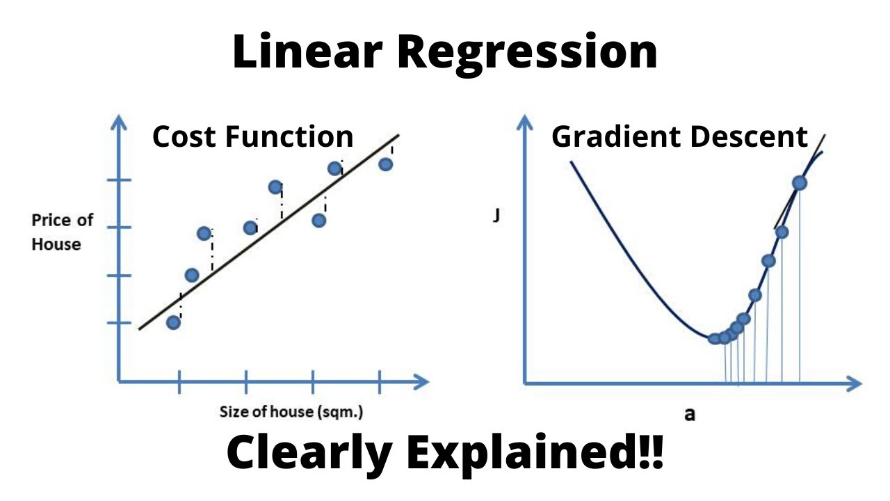
Linear Regression, Cost Function and Gradient Descent Algorithm..Clearly Explained !!
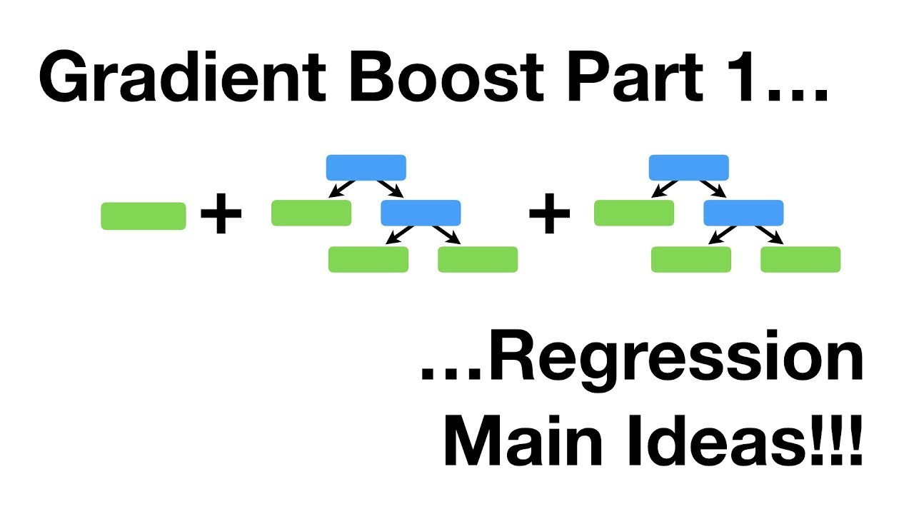
Gradient Boost Part 1 (of 4): Regression Main Ideas
5.0 / 5 (0 votes)