How to Create MIS Report in excel | Impressive and Interactive MIS Report In Excel | Simplilearn
Summary
TLDRThis video from Simply Learn's YouTube channel offers a comprehensive tutorial on creating MIS (Management Information System) reports using Excel. It explains the significance of MIS reports in aiding management decisions and walks through the process of building interactive reports with pivot tables, pivot charts, and slicers. The tutorial covers step-by-step instructions on setting up various charts (like bar and pie charts), ensuring proper connections between slicers and charts, and handling complex datasets. Viewers are also reminded to disable macros and convert data to table format for optimal results.
Takeaways
- 📊 MIS stands for Management Information System and is used for generating reports in Excel to aid in decision-making.
- 💼 MIS reports provide data across various categories, helping management assess organizational performance for better decision-making.
- 🖥️ The process of creating MIS reports in Excel involves using tools like pivot tables to generate interactive reports.
- 📈 Pivot tables and pivot charts in Excel are essential for organizing and visualizing data for MIS reports.
- 🔄 Slicers in Excel allow users to filter data dynamically, making reports more interactive and providing real-time insights.
- 🚗 In the example, sales data from car manufacturers (like BMW) is used to demonstrate MIS report creation, showcasing pivot tables and slicers.
- 📑 To create a pivot table, you need to select data, insert a pivot table, and then drag fields into rows, columns, and values to build the report.
- 📊 Pivot charts (like column, pie, and bar charts) help visualize data from pivot tables, making reports more understandable.
- 🛠️ When using multiple pivot charts, it's important to connect slicers to all charts to ensure synchronization when filtering data.
- ✅ To effectively work with Excel MIS reports, it's crucial to disable macros and convert data into table format using the Ctrl+T shortcut.
Q & A
What is an MIS report in Excel?
-MIS stands for Management Information System. An MIS report in Excel provides data on different categories to aid accurate decision-making. It helps management assess the performance of an organization and supports faster decision-making.
How can MIS reports in Excel be useful for job opportunities?
-Knowing how to create MIS reports using business intelligence tools like Excel can help you find good job opportunities in established companies, as it’s a valuable skill for data management and decision-making processes.
What is the process of creating a pivot table in Excel?
-To create a pivot table in Excel, select the data range, go to the 'Insert' ribbon, and choose the 'Pivot Table' option. Select whether you want to create the table in the same sheet or a new one, and then drag fields into the rows, columns, and values areas to organize the data.
What are slicers, and how are they used in Excel?
-Slicers are interactive filters in Excel that allow users to quickly filter data in pivot tables and charts. In the tutorial, slicers are used to filter data by year, company, and type of car to get real-time information from the dashboard.
How do you create a pivot chart in Excel?
-After creating a pivot table, you can create a pivot chart by selecting the entire data in the pivot table, going to the 'Insert' tab, and choosing 'Pivot Chart'. You can then select different chart types, such as column, pie, or bar charts, to represent the data visually.
What should you do if only one chart is interacting with the slicer in a dashboard?
-If only one chart is interacting with a slicer, you need to connect the slicer to all relevant pivot tables. Right-click the slicer, select 'Report Connections,' and connect it to all the necessary pivot tables.
Why is it important to convert your data into tabular form in Excel?
-It’s important to convert data into tabular form because Excel treats tabular data more efficiently for creating MIS reports and pivot tables. It also ensures that macros are disabled and the data is in the proper format for analysis.
What steps are needed to convert data into tabular form in Excel?
-To convert data into tabular form, select the entire data set, press 'Ctrl + T', and ensure the 'My table has headers' option is selected. This will structure the data in a table format with clear headers.
What are some common chart types used in MIS reports in Excel?
-Common chart types used in MIS reports include column charts, pie charts, and bar charts. These visual representations help to better illustrate and compare data for management analysis.
What should you do if you want to move a chart to another worksheet in Excel?
-To move a chart to another worksheet, right-click the chart, select 'Pivot Chart Analyze,' choose the 'Move Chart' option, and then select the destination worksheet where you want the chart to be displayed.
Outlines

Esta sección está disponible solo para usuarios con suscripción. Por favor, mejora tu plan para acceder a esta parte.
Mejorar ahoraMindmap

Esta sección está disponible solo para usuarios con suscripción. Por favor, mejora tu plan para acceder a esta parte.
Mejorar ahoraKeywords

Esta sección está disponible solo para usuarios con suscripción. Por favor, mejora tu plan para acceder a esta parte.
Mejorar ahoraHighlights

Esta sección está disponible solo para usuarios con suscripción. Por favor, mejora tu plan para acceder a esta parte.
Mejorar ahoraTranscripts

Esta sección está disponible solo para usuarios con suscripción. Por favor, mejora tu plan para acceder a esta parte.
Mejorar ahoraVer Más Videos Relacionados
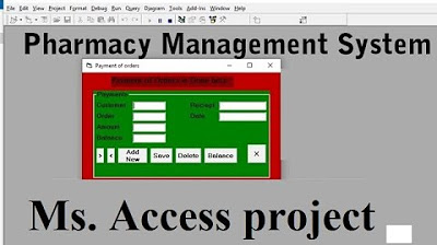
Pharmacy Management System using Microsoft Access

Coding Interview Questions And Answers | Programming Interview Questions And Answers | Simplilearn

What Is An Algorithm? | What Exactly Is Algorithm? | Algorithm Basics Explained | Simplilearn

Cara Menggunakan Accurate Online untuk Pemula ‼️
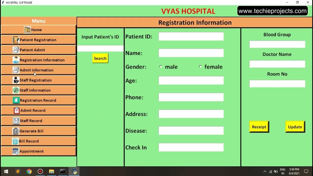
Hospital Management System in Python with MySQL Connectivity

Performance Testing Tutorial For Beginners | Performance Testing Using Jmeter | Simplilearn
5.0 / 5 (0 votes)
