Linear Regression, Cost Function and Gradient Descent Algorithm..Clearly Explained !!
Summary
TLDRThis video introduces linear regression, a fundamental machine learning model used to predict outputs based on input features. It explains the concept of a model in data science, the importance of understanding and predicting real-world processes, and how linear regression works with a single feature. The video also covers multiple feature linear regression, the cost function, and the gradient descent algorithm for finding the best model parameters. It concludes with practical insights on implementing linear regression in Python and the significance of the learning rate as a hyperparameter.
Takeaways
- 🧠 A model in data science is a mathematical representation of a real-world process, focusing on the relationship between inputs and outputs.
- 🔮 Models are valuable for understanding processes and predicting outcomes based on input features, which can have significant economic benefits.
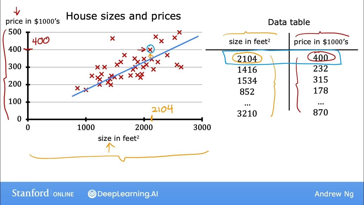
- 🏠 The example of house size predicting its price illustrates the use of a simple linear model where input (size) determines output (price).
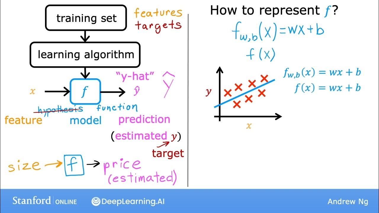
- 📊 Linear regression is introduced as a method to find a linear relationship between input features and an output variable, represented graphically on a coordinate plane.
- 🔢 The equation of a linear relationship is expressed as y = a0 + a1*x, where y is the output, x is the input feature, and a0 and a1 are model parameters.
- 📈 For multiple features, the linear equation extends to y = a0 + a1*x1 + a2*x2 + ... + an*xn, with each xi representing a feature and ai the corresponding model parameter.
- 📉 The cost function, derived from the sum of squared errors (SSE), is used to measure how well the model fits the data and guides the model parameter adjustments.
- 🔍 The gradient descent algorithm is employed to minimize the cost function by iteratively adjusting model parameters based on the slope (derivative) of the cost function.
- 🔄 The learning rate (alpha) in gradient descent determines the size of the steps taken towards the minimum of the cost function, requiring careful tuning to ensure convergence.
- 💻 Linear regression models can be implemented in Python with libraries that abstract the complex mathematics, allowing for efficient model training and prediction.
Q & A
What is a model in the context of data science?
-In data science, a model is a mathematical representation of a real-world process, characterized by an input-output relationship.
Why are models important in data science?
-Models are important because they help us understand the nature of the process being modeled and enable us to predict outputs based on input features, which has significant economic value.
What is linear regression and why is it significant?
-Linear regression is a machine learning model used to establish a linear relationship between a dependent variable and one or more independent variables. It's significant because it provides a simple and effective way to predict outcomes based on input features.
How is the relationship between house size and price represented in linear regression?
-In linear regression, the relationship between house size (input) and price (output) is represented as a straight line on a graph, where the x-axis represents the size of the house and the y-axis represents the price.
What are the model parameters in a simple linear regression model?
-In a simple linear regression model, the model parameters are 'a naught' (intercept) and 'a1' (coefficient), which define the equation of the line as 'y = a naught + a1 * x'.
How does the cost function in linear regression work?
-The cost function in linear regression measures the difference between the predicted values and the actual values. It is typically represented as the sum of the squares of the differences (errors) between predicted and actual values, divided by the number of examples (m).
What is the purpose of the gradient descent algorithm in linear regression?
-The gradient descent algorithm is used to minimize the cost function in linear regression by iteratively adjusting the model parameters (a naught and a1) to find the values that result in the lowest cost.
How does the learning rate (alpha) affect the gradient descent process?
-The learning rate (alpha) determines the size of the steps taken towards the minimum of the cost function during each iteration of gradient descent. A higher learning rate can lead to faster convergence but might cause the algorithm to overshoot the minimum, while a lower learning rate ensures a more stable convergence but may slow down the process.
What is the role of the error term in the cost function?
-The error term (e) in the cost function represents the difference between the actual value and the predicted value for each training example. It is used to calculate the cost, which is then minimized through the gradient descent process.
How can linear regression be extended to handle multiple features?
-Linear regression can be extended to handle multiple features by including additional terms in the equation, each multiplied by its respective feature (x1, x2, ..., xn) and coefficient (a1, a2, ..., an), allowing the model to capture more complex relationships.
What is the significance of the intercept (a naught) in a linear regression model?
-The intercept (a naught) in a linear regression model represents the expected value of the dependent variable when all the independent variables are set to zero. It helps to position the regression line on the y-axis.
Outlines
📊 Introduction to Linear Regression
The video begins by introducing the concept of linear regression as the first machine learning model. It explains that a model in data science is a mathematical representation of a real-world process, focusing on the input-output relationship. The video uses the example of pizza slices eaten based on the time since the last meal to illustrate a simple model. It emphasizes the importance of models in understanding processes and predicting outcomes, highlighting the economic value of predictive capabilities. The concept is further explored through the example of predicting house prices based on size, introducing the idea of training examples and the linear relationship between input features and output targets. The video then delves into the linear equation representing this relationship, explaining how multiple features can be incorporated into the model. It sets the stage for discussing how to find the best-fitting line through the data, introducing the cost function as a metric for evaluating model fit.
🔍 Minimizing Error with Gradient Descent
The second paragraph delves into the process of finding the best model parameters using the gradient descent algorithm. It starts by discussing how different combinations of model parameters affect the cost function, which is a measure of the model's accuracy. The video uses a graphical representation to explain how the algorithm works, moving towards the minimum of the cost function by adjusting parameters based on the slope (derivative) at each step. The learning rate, a key hyperparameter, is introduced as a factor controlling the size of these steps. The video warns about the potential pitfalls of setting the learning rate too high, which can cause the algorithm to overshoot the minimum and fail to converge. It concludes by emphasizing that while understanding the theory behind the cost function and gradient descent is important, practical implementation can be done with just a few lines of code in Python, thanks to inbuilt packages that handle the mathematical complexities. The video also touches on the importance of choosing the right learning rate to ensure efficient and accurate model training.
Mindmap
Keywords
💡Model
💡Linear Regression
💡Cost Function
💡Gradient Descent
💡Training Examples
💡Features
💡Target Variable
💡Parameters
💡Learning Rate
💡Hyperparameters
Highlights
A model in data science is a mathematical representation of a real-world process.
Models help us understand and predict the output based on input features.
Linear regression is introduced as the first machine learning model to learn.
Linear relationships between variables can be represented as a straight line equation.
The model parameters are crucial for fitting a line to the data points.
Multiple features can be incorporated into the linear equation.
The cost function, or error metric, is used to judge the best fit line.
Gradient descent algorithm is used to minimize the cost function.
The learning rate is a critical hyperparameter in gradient descent.
The slope of the cost function at a point determines the direction of the next step in gradient descent.
The size of steps in gradient descent is dependent on the slope of the cost function.
The iterations of gradient descent continue until the cost function is minimized.
Linear regression can be easily implemented in Python with inbuilt packages.
The learning rate should be carefully chosen to ensure convergence of the algorithm.
Understanding the theory behind the cost function and gradient descent is essential for training linear regression models.
The video concludes with a congratulatory message for understanding the first machine learning model.
Transcripts
[Music]
hello and welcome
today we'll learn about linear
regression our first machine learning
model
what is a model
i know what you're thinking but that's
not the kind of model we generally refer
to in data science
a model is basically a mathematical
representation of a real-world process
in the form of input output relationship
something like this
slices of pizza i'll eat my output will
be determined by r since my last meal
which is input that means if it is two
hours since my last meal i can eat five
slices of freezer
even though it is useless this is an
example of simple model
but why should someone make models
not only models help us understand the
nature of the process being modeled they
also enable us to predict the output
based on the input features and the
ability to predict the unknown has great
economic value
let's look at an example
this is size of a house and this is
corresponding price of that house
these are observations for individual
houses also known as training examples
now we want to know price of a new house
which will be output of our model based
on its size which is input
to start looking for a simple and yet
effective model for this problem our
first stop would be linear regression
can't believe this is the same problem
it looks good on graph
so on x axis we have our input size of
house and on y-axis the output its price
any linear relationship between two
variables can be represented as a
straight line whose equation can be
written as y equals a naught plus a1 x
where y is output or target
which is price of house in our case and
x is input of feature which is size of
house
and a node and a1 are model parameters
but what if there are more than one
feature
any general linear equation with
multiple features can be written as
y equals a naught plus a 1 x 1 plus a 2
x 2 and so on up to a and x m
where x i's that are
x 1 x 2 till xn are features ai's that
is a naught a 1 and so on till a n are
modern parameters and y is target
variable
as per our linear regression model we
need to fit a straight line to it with
equation y equals a naught plus a 1 x
and depending on values of a naught and
a 1 we can have many possibilities which
look promising
we need to settle the case on a value of
parameters a naught and a 1
corresponding to which straight line
fits best to the data
for this we need to agree on a metric to
judge best fit and we can choose that
straight line which performs best on
that metric first function to the rescue
let's suppose we have m training
examples or observations and this is the
first one
this is our model
from this we know that this is actual
price of first example and this is price
of first example as predicted by a model
which falls on a straight line for that
size
let's call this difference as error term
e which is like y actual minus y
predicted
since it is for first example let's call
it even
for ith example we define error term as
e i equals y predicted minus y actual
now as you might have understood ei can
be positive or negative depending on
whether y actual is more or y predicted
we will square e i's to make it positive
so the order doesn't matter
cos function will be defined as 1 by 2 m
even square plus e 2 square and so on
till e m square
where m is the number of examples
and e i's are error terms
we can also write it as 1 by 2 m
summation of
y predicted minus y actual square
we just expanded e is to y predicted
minus y actually we can also write it as
1 by 2 m summation of a naught plus a 1
x 1 minus y actual square
we just expanded y predicted which is a
naught plus a 1 x 1 as per our model
clearly cos function j is a function of
parameter space a naught and a1
i think you would have guessed it by now
the best fitting model would be the one
which minimizes our error metric which
is cos function
such a straight line will be the best
linear approximation of the linear
relationship between house price and
size of the house
another interpretation of cost function
can be the measure of distance of our
model from data points lesser the
distance better is our model
now we just need to minimize cost
function but how to do that
we have established the fact that all
the straight lines are just different
combination of model parameters a naught
and a1
and cost function is a function of
parameter space as well
therefore by changing a naught and a1 we
can change the cost function we will
keep changing a naught and a1 till we
find a combination where cos function is
minimized
and for this we will take help of
gradient descent algorithm
let's just forget cost function for some
time assume a function any regular
function j equals f of a
this curve of j
represent the values j will assume for
different values of a
indeed that is what makes it a function
of a
we are at this point now a1 and f a1
and we want to reach here we want to
know for what value of a a function will
assume minimum
how can we reach minimum starting from
a1
[Music]
let's calculate stop slope at this point
a1 f of a
it is dj by da at a1 or m dash a1
don't worry if you don't understand dj
by da you can interpret it as a slope at
that point
let's move a step alpha in that
direction to reach a1 minus alpha times
after shape
alpha is a small fixed quantity in the
range of 0.01 therefore the size of our
steps is dependent on the slope f dash
a1 higher the value of slope which
occurs away from minima larger the steps
and vice versa
as we move closer to the minima the
slope decreases and hence our steps
towards minimum keeps on getting smaller
at minimum slope becomes zero
these iteration of gradient descent
algorithm can run in thousands or tens
of thousands depending on nature of
function our learning rate and of course
where we start from even in this space
we will use the same methodology to
minimize cost function
which is a function of model parameters
a naught and a1
by changing them through iteration of
gradient descent alcohol
this is the part where it can get too
mathematical for some people but don't
worry if you don't get it completely
you'll be working just fine without it
as well
step one in gradient descent algorithm
would be to calculate slope with respect
to both parameters separately at the
current or initial value of parameters a
naught and a1
next we need to take the step alpha and
update the new parameters as follows
third step would be to update the cost
function
with new a naught and a1 and then repeat
the step one
these iterations should be run thousands
of times
we can easily scale this for multiple
features
as you know our equation of linear
regression for multiple features is y
equals a naught plus a1 x1 plus a2 x2
and so on till a and x
we just have to update all the model
parameters by calculating slope and then
implementing gradient descent steps for
every parameter simultaneously
understanding theory behind cos function
and gradient descent algorithm was
essential but as we shall see we can
train linear regression model with just
few lines of code and python
these are inbuilt packages
which implement all of this in an
optimized way so that we don't have to
worry about all the maths behind it
one important thing to understand about
gradient descent is the learning rate
alpha
we know that step taken towards the
minima was alpha times f dash
so as we increase learning rate we will
take larger step towards minimum and
hence we will reach minimum early this
will make our algorithm fast right
let's suppose we set alpha 200
and we reach here in a step from a1 by
setting alpha to 100
can you guess what can potentially
happen in the next iteration
it will fail to converge to minimum and
will keep on oscillating around minimum
but can never converge even in a billion
iteration so what is the solution
keep alpha smart
its value is kept around 0.01
so that it neither makes gradient
descent too slow nor does it fail to
converge
learning rate alpha is hyper parameter
for this model
even though it doesn't directly affect
model like parameters a1 a naught and a1
do but it can impact performance of our
model and we need to be cautious about
choosing model hyper parameters
that's all about linear regression
congrats on understanding your first ml
model
please like this video if you found it
useful and if you have any doubt please
raise them in the comment section thanks
for watching
[Music]
Ver Más Videos Relacionados
#10 Machine Learning Specialization [Course 1, Week 1, Lesson 3]
Gradient Descent, Step-by-Step
Machine Learning Tutorial Python - 8: Logistic Regression (Binary Classification)
Lec-3: Introduction to Regression with Real Life Examples
Lec-4: Linear Regression📈 with Real life examples & Calculations | Easiest Explanation
#9 Machine Learning Specialization [Course 1, Week 1, Lesson 3]
5.0 / 5 (0 votes)