26 - Denoising and edge detection using opencv in Python
Summary
TLDRIn this Python tutorial, Trini from the 'Python for Microscopists' YouTube channel explores OpenCV's image processing capabilities, focusing on denoising and edge detection. She demonstrates various blurring techniques like averaging, Gaussian blur, and custom filters, emphasizing the importance of kernel size. Trini also introduces edge detection using the Canny algorithm, showcasing its effectiveness in identifying image edges. The tutorial is aimed at those interested in pre-processing microscope images for tasks like segmentation and object detection.
Takeaways
- 😀 The tutorial focuses on OpenCV, a library used for machine vision and image processing, including microscope images.
- 🔍 Denoising and blurring are discussed as important pre-processing steps for image segmentation.
- 💻 The IDE used is part of the Anaconda distribution, and OpenCV, NumPy, and Matplotlib are the primary libraries imported.
- 📸 The image 'BSC_Google_9e.jpg' is used as an example, which is a microscope image with added noise.
- 🛠️ Denoising methods include averaging, Gaussian blur, and median filtering, which are performed by convolving an image with a kernel.
- 📊 A custom 5x5 kernel is created using NumPy, normalized to maintain the original image's energy.
- 🔧 The cv2.filter2D function is used for custom filtering, and cv2.blur and cv2.GaussianBlur are used for built-in blurring techniques.
- 📈 The tutorial compares different denoising methods, highlighting the effectiveness of Gaussian blur and median filtering in retaining edges.
- 👁️🗨️ Bilateral filtering is introduced as a favorite method for noise removal while preserving edges, which is crucial for microscope images.
- 🏞️ Edge detection is covered, with a focus on the Canny edge detection method, which is useful for identifying significant transitions in images.
Q & A
What are the two main topics discussed in the Python tutorial video by Trini?
-The two main topics discussed are denoising or blurring and edge detection, which are important pre-processing operations for image segmentation.
Why is OpenCV used in the tutorial?
-OpenCV is used because it is a library primarily dedicated to machine vision applications and has very good tools for image processing, including microscope images.
What is the purpose of importing NumPy in the context of this tutorial?
-NumPy is imported for array manipulations, specifically to generate a matrix for defining a kernel used in the denoising process.
How does the denoising process work in the tutorial?
-Denoising involves manipulating the image using a kernel to reduce noise. This can be done through averaging, Gaussian blur, or other filtering techniques like median or bilateral filtering.
What is the significance of normalizing the kernel by dividing it by 25 in the tutorial?
-Normalizing the kernel by dividing it by 25 ensures that the total energy of the image is not altered during the convolution process, maintaining the original image's characteristics.
Why is a 5x5 kernel used in the denoising example?
-A 5x5 kernel is used to apply a larger area of averaging, which can be more effective in reducing noise while preserving image details compared to smaller kernels.
What is the difference between the custom filter and the Gaussian blur in the tutorial?
-The custom filter uses a simple averaging method with an all-ones kernel, while Gaussian blur uses a kernel with values that decrease based on the distance from the center, emulating a bell curve.
How does the median filter help in retaining edges during denoising?
-The median filter retains edges by replacing the central pixel value with the median of the pixel values in the kernel, which is effective in removing noise while preserving edges.
What is the bilateral filter and why is it one of Trini's favorite filters?
-The bilateral filter is a non-linear, edge-preserving, and noise-reducing smoothing filter. It is favored because it effectively removes noise while keeping edges sharp, which is crucial for image processing tasks like image segmentation.
What is the Canny edge detection method and how is it used in the tutorial?
-The Canny edge detection method is an edge detection operator that uses a multi-stage algorithm to detect a wide range of edges in images. In the tutorial, it is used to highlight the edges of a neuron in a microscope image.
What are the next steps in image processing after denoising and edge detection as suggested by Trini?
-After denoising and edge detection, the next steps suggested are image thresholding and segmentation, which are further pre-processing operations leading to more advanced image analysis.
Outlines

Esta sección está disponible solo para usuarios con suscripción. Por favor, mejora tu plan para acceder a esta parte.
Mejorar ahoraMindmap

Esta sección está disponible solo para usuarios con suscripción. Por favor, mejora tu plan para acceder a esta parte.
Mejorar ahoraKeywords

Esta sección está disponible solo para usuarios con suscripción. Por favor, mejora tu plan para acceder a esta parte.
Mejorar ahoraHighlights

Esta sección está disponible solo para usuarios con suscripción. Por favor, mejora tu plan para acceder a esta parte.
Mejorar ahoraTranscripts

Esta sección está disponible solo para usuarios con suscripción. Por favor, mejora tu plan para acceder a esta parte.
Mejorar ahoraVer Más Videos Relacionados

25 - Reading Images, Splitting Channels, Resizing using openCV in Python
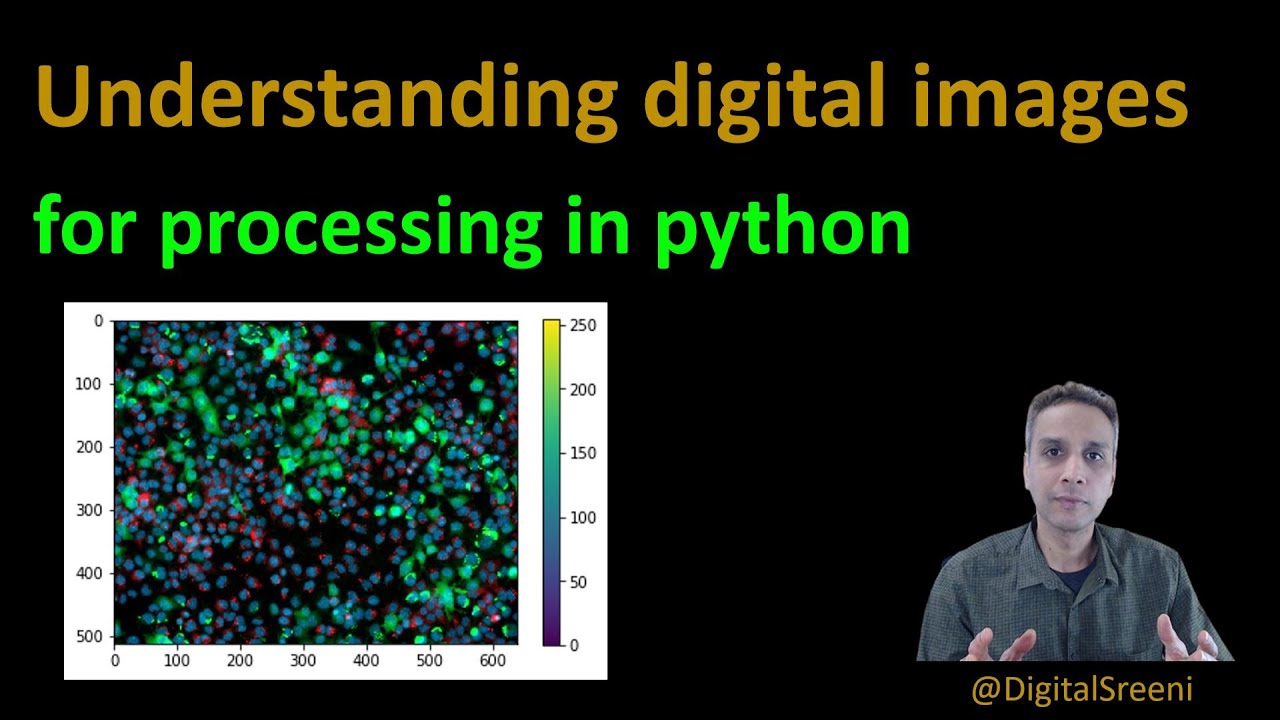
16 - Understanding digital images for Python processing

Cartoon Effect on Image using OpenCV | Machine Learning Project 8 | ML Training | Edureka
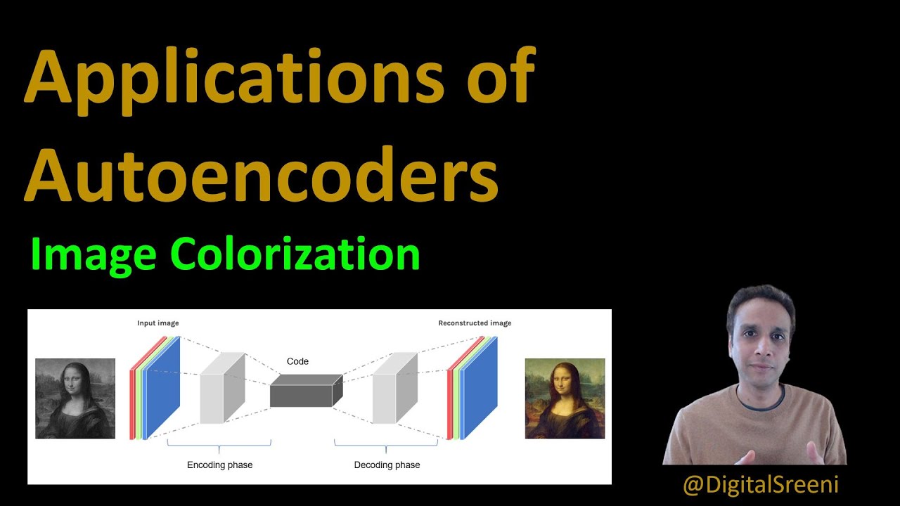
90 - Application of Autoencoders - Image colorization

OpenCV on Google Colab - Working with Gray Image

Lesson 7-2: String Indexing and Slicing
5.0 / 5 (0 votes)
