Introduction to Operational Amplifier: Characteristics of Ideal Op-Amp
Summary
TLDRThis video from the 'All About Electronics' YouTube channel introduces the operational amplifier (op-amp), a high-gain differential amplifier used for amplifying input signals and performing mathematical operations like addition, subtraction, integration, and differentiation. The script explains the op-amp's circuit symbol, input terminals, and the concept of open-loop gain. It also covers the saturation behavior of the op-amp and its applications in various electronic circuits, highlighting the importance of choosing the right op-amp based on specific characteristics like slew rate and common mode rejection ratio for different applications.
Takeaways
- 😀 The video introduces the concept of an operational amplifier (op-amp), which is a high-gain amplifier used to amplify input signals.
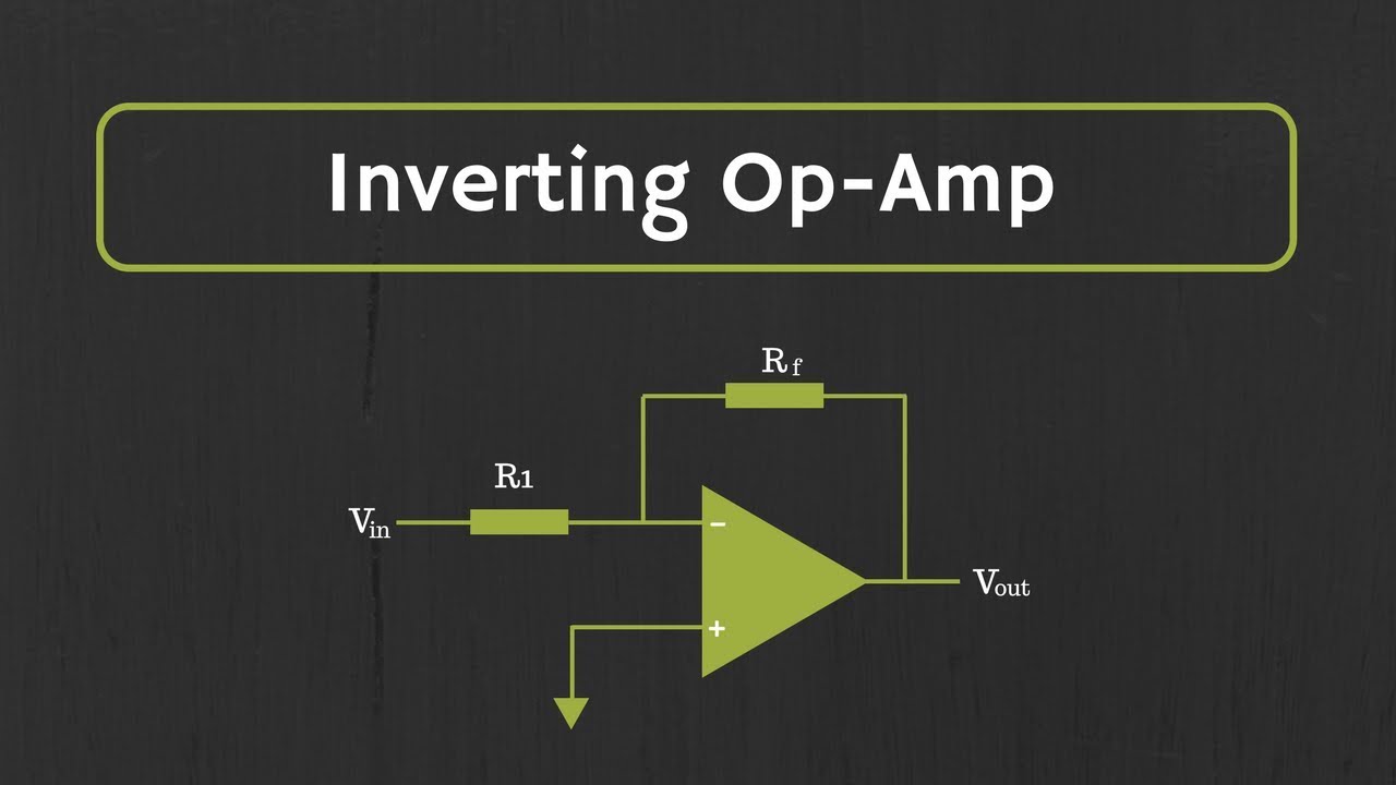
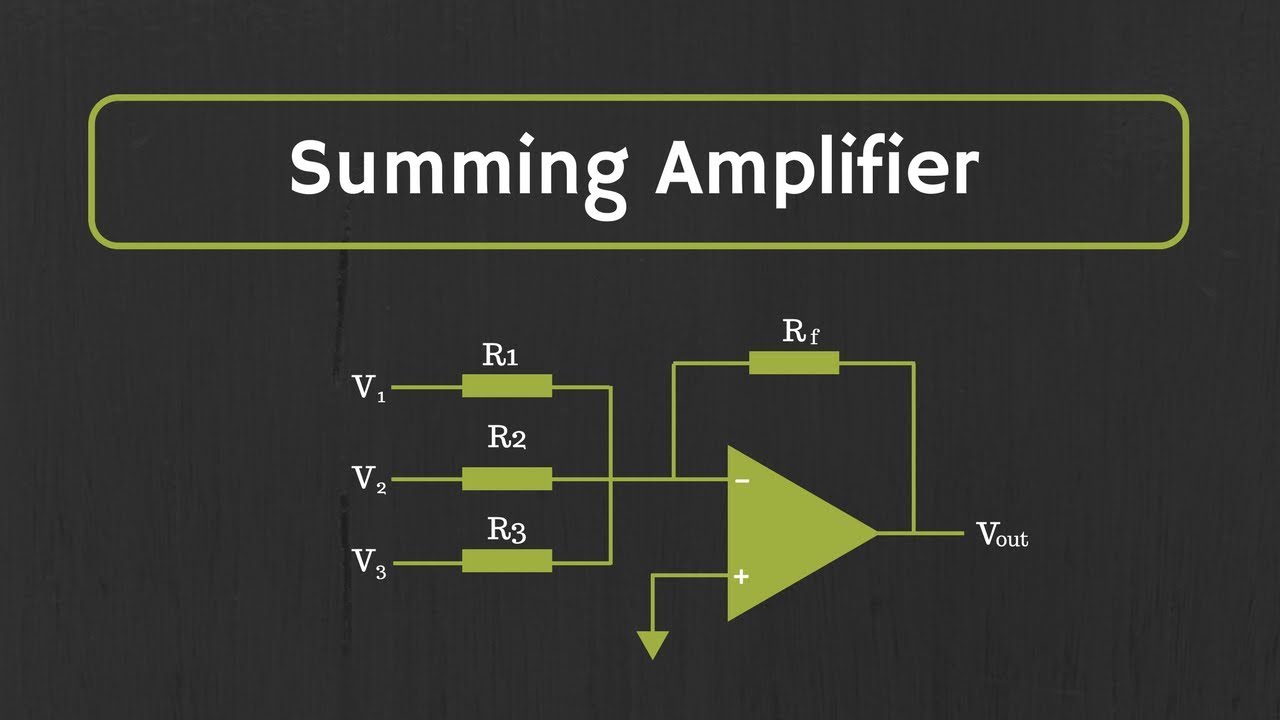
- 🔍 The term 'operational amplifier' originates from its early use in performing mathematical operations such as addition, subtraction, integration, and differentiation.
- 🔌 The op-amp typically has two inputs (non-inverting and inverting) and one output, and can operate with either dual power supplies or a single power supply.
- 📶 The operational amplifier functions as a differential amplifier, amplifying the difference between the two input signals, with the output being proportional to the gain (A) times the difference of the inputs (V1 - V2).
- 🔄 The open-loop gain of an op-amp refers to its gain without any feedback, which can be extremely high, in the range of 10^5 to 10^6.
- 🔁 The op-amp's output is restricted by the biasing voltages and will saturate at certain levels, which is useful for comparator applications.
- 🛠️ The op-amp is a versatile component found in various applications, including active filters, oscillators, waveform converters, and analog-to-digital converters.
- 📊 The voltage transfer curve of an op-amp shows the relationship between the differential input and the output voltage, highlighting the gain and saturation points.
- 🌐 The ideal op-amp is characterized by infinite input impedance, zero output impedance, infinite bandwidth, infinite gain, and infinite slew rate, with zero output when input is zero.
- 🔄 Slew rate is the measure of how quickly an op-amp can respond to changes in input voltage, particularly important for square wave inputs.
- 🔄 Common mode rejection ratio (CMRR) is a parameter that indicates how well an op-amp can reject common input voltages and amplify the difference between the two inputs, with an ideal op-amp having an infinite CMRR.
Q & A
What is an operational amplifier (op-amp)?
-An operational amplifier, or op-amp, is a type of amplifier that amplifies the difference between two input signals. It is a versatile integrated circuit used in various applications like signal amplification, mathematical operations, filters, oscillators, and more.
Why is it called an 'operational' amplifier?
-The op-amp is called an 'operational' amplifier because, before digital computers, it was used to perform various mathematical operations such as addition, subtraction, integration, and differentiation by connecting a few resistors and capacitors.
What are the two input terminals of an op-amp called, and what do they represent?
-The two input terminals of an op-amp are called the non-inverting input (marked with a positive sign) and the inverting input (marked with a negative sign). The non-inverting input produces an output in phase with the input, while the inverting input produces an output that is 180 degrees out of phase with the input.
What is meant by the 'open-loop gain' of an op-amp?
-The open-loop gain of an op-amp refers to the gain of the amplifier when there is no feedback loop from the output to the input. It is typically very high, ranging from 100,000 (10^5) to 1,000,000 (10^6).
How does the op-amp output behave when a small input signal is applied in an open-loop configuration?
-In an open-loop configuration, even a small input signal can cause the op-amp's output to saturate, reaching the positive or negative biasing voltage limits, depending on the input signal's polarity.
What are some common applications of op-amps?
-Op-amps are used in a variety of applications, including comparators, active filters, oscillators, waveform converters, analog-to-digital converters, and digital-to-analog converters.
What are the ideal characteristics of an op-amp?
-The ideal op-amp has infinite input impedance, zero output impedance, infinite open-loop gain, infinite bandwidth, and infinite slew rate. Additionally, when the input voltage is zero, the output should also be zero, and it should have an infinite common-mode rejection ratio.
What is slew rate in the context of an op-amp, and why is it important?
-The slew rate of an op-amp is the rate at which the output voltage can change in response to a step input voltage. It is usually expressed in volts per microsecond (V/µs). A high slew rate is important for accurately reproducing fast-changing signals, such as square waves.
What is the common-mode rejection ratio (CMRR) in an op-amp?
-The common-mode rejection ratio (CMRR) is a measure of an op-amp's ability to reject common-mode signals, which are the same at both input terminals, while amplifying the differential signal, which is the difference between the two input voltages. Ideally, the CMRR should be infinite.
How do practical op-amps differ from ideal op-amps?
-Practical op-amps have finite input and output impedances, a finite open-loop gain, and non-infinite bandwidth and slew rate. They may also have a small output even when the input is zero, known as offset voltage, and their CMRR is finite.
Outlines

Dieser Bereich ist nur für Premium-Benutzer verfügbar. Bitte führen Sie ein Upgrade durch, um auf diesen Abschnitt zuzugreifen.
Upgrade durchführenMindmap

Dieser Bereich ist nur für Premium-Benutzer verfügbar. Bitte führen Sie ein Upgrade durch, um auf diesen Abschnitt zuzugreifen.
Upgrade durchführenKeywords

Dieser Bereich ist nur für Premium-Benutzer verfügbar. Bitte führen Sie ein Upgrade durch, um auf diesen Abschnitt zuzugreifen.
Upgrade durchführenHighlights

Dieser Bereich ist nur für Premium-Benutzer verfügbar. Bitte führen Sie ein Upgrade durch, um auf diesen Abschnitt zuzugreifen.
Upgrade durchführenTranscripts

Dieser Bereich ist nur für Premium-Benutzer verfügbar. Bitte führen Sie ein Upgrade durch, um auf diesen Abschnitt zuzugreifen.
Upgrade durchführenWeitere ähnliche Videos ansehen
Operational Amplifier: Inverting Op Amp and The Concept of Virtual Ground in Op Amp
Op-Amp: Summing Amplifier (Inverting and Non-Inverting Summing Amplifiers)
What is an operational amplifier?
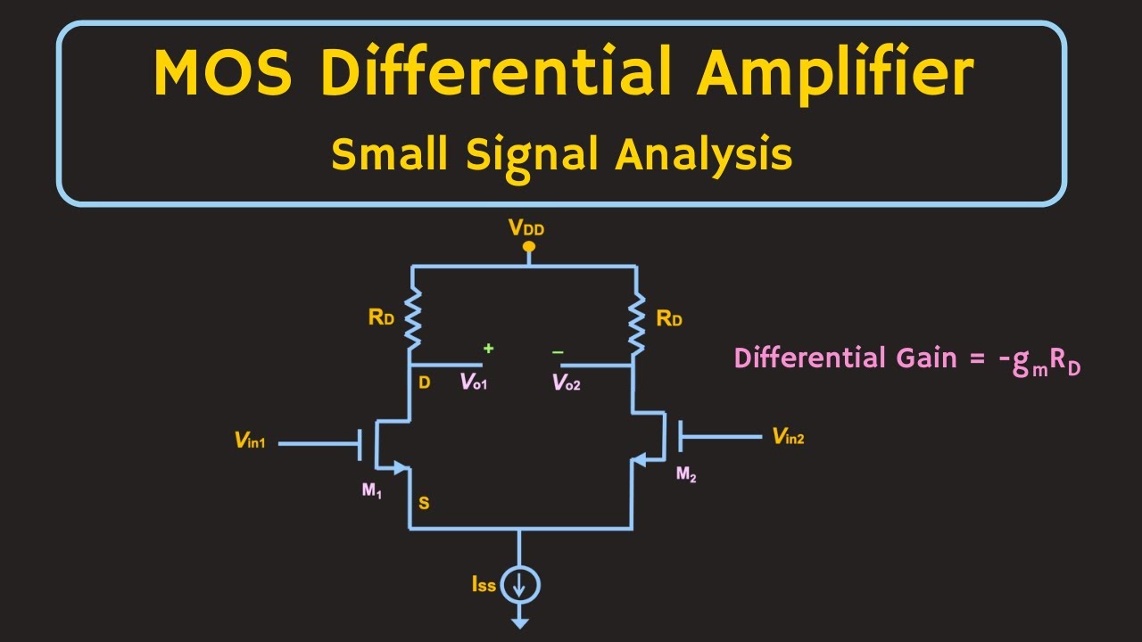
MOSFET - Differential Amplifier (Small Signal Analysis)
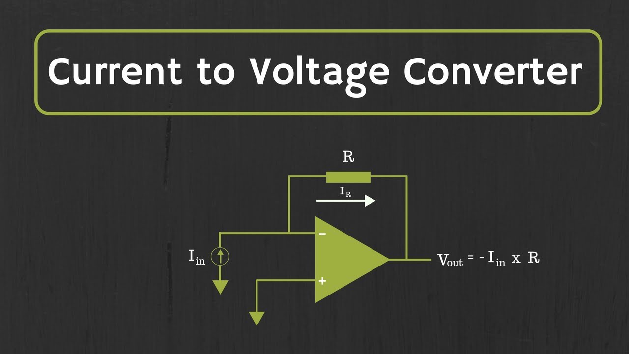
Op-Amp: Current to Voltage Converter (Transimpedance Amplifier) and it's applications

Operational Amplifier: Op-Amp as Differential Amplifier or Op-Amp as subtractor (With Examples)
5.0 / 5 (0 votes)
