Normal Distribution: Calculating Probabilities/Areas (z-table)
Summary
TLDRThis video tutorial demonstrates how to use standard normal distribution tables to calculate probabilities. It explains the concept of a z-score, which measures how many standard deviations a data point is from the mean. The script guides through examples of finding probabilities for scores below a certain value, above another, and between two values. It concludes with the method to determine 'less than', 'greater than', and 'between' areas using cumulative tables, emphasizing the importance of subtracting areas, not z-values, for the latter.
Takeaways
- 📚 The video explains how to use standard normal distribution tables to calculate probabilities.
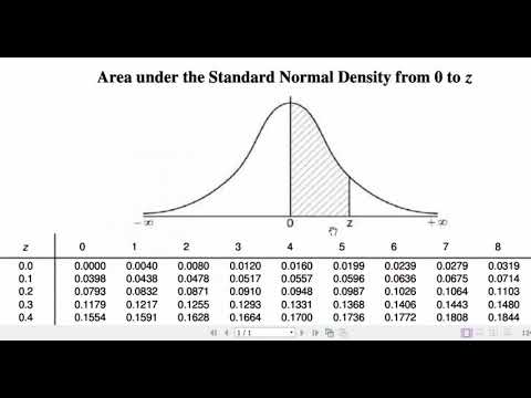
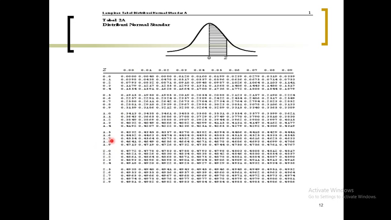
- 📉 A normal distribution is symmetric and bell-shaped, with the total area under the curve equaling 1 or 100%.
- 📍 The standard normal distribution has a mean (µ) of 0 and a standard deviation (σ) of 1.
- 🔄 The formula to convert any score x from a normal distribution to a standard normal score (z-score) is z = (x - µ) / σ.
- 📊 The z-score represents how many standard deviations a score is from the mean.
- 🔑 The video uses 'Less Than' cumulative tables for standard normal distribution, which are typically shaded for the left tail.
- 🔍 For a given exam score example, the z-score for x = 54 is calculated as -1.22 (rounded from -1.2222).
- 📌 The probability that a score is less than 54 is found by looking up the area to the left of z = -1.22 in the table, which is 0.1112 or 11.12%.
- 🚫 In continuous distributions like the normal distribution, 'at least' and 'greater than' are treated the same for probability calculations.
- 🔢 For the exam example, the probability that a score is at least 80 is calculated by subtracting the area to the left of z = 1.67 from 1, resulting in 0.0475 or 4.75%.
- 🌐 To find the probability of a score being between two values, subtract the area to the left of the smaller z-score from the area to the left of the larger z-score, as demonstrated with the range between 70 and 86.
Q & A
What is a normal distribution?
-A normal distribution is a symmetric, bell-shaped distribution where the area under the curve is 1 or 100%, representing the probability of all possible outcomes.
What distinguishes a standard normal distribution from other normal distributions?
-A standard normal distribution, also known as the z-distribution, has a mean (µ) of 0 and a standard deviation (σ) of 1, making it a special case of the normal distribution.
What is the formula to convert a score from any normal distribution to a standard normal score?
-The formula to convert a score x from any normal distribution to a standard normal score, also known as the z-score, is z = (x - µ) / σ.
What are the 'Less Than' cumulative tables used for in the context of standard normal distribution?
-The 'Less Than' cumulative tables are used to find the probability of a score being less than a certain value in a standard normal distribution by looking up the corresponding z-score.
How do you calculate the z-score for a score of 54 given a mean of 65 and a standard deviation of 9?
-To calculate the z-score for a score of 54, you subtract the mean (65) from the score (54) and then divide by the standard deviation (9), which results in a z-score of -1.2222, rounded to -1.22 for table lookup.
What is the probability that a score is less than 54 given the same distribution as in the example?
-The probability that a score is less than 54 is found by looking up the corresponding z-score of -1.22 in the standard normal table, which gives an area of 0.1112 or 11.12%.
How does the concept of 'at least' relate to 'greater than' in continuous distributions like the normal distribution?
-In continuous distributions, such as the normal distribution, 'at least' and 'greater than' are treated the same because the probability of a score being exactly at a certain value is zero.
What is the probability that a score is at least 80 given the exam scores distribution in the example?
-The probability that a score is at least 80 is found by looking up the z-score of 1.67 in the standard normal table, which gives an area of 0.9525. Subtracting this from 1 gives 0.0475 or 4.75%.
How do you calculate the probability of a score falling between two values, such as 70 and 86, in the given distribution?
-To find the probability of a score falling between 70 and 86, calculate the z-scores for both values, look up the corresponding areas in the standard normal table, and subtract the smaller area from the larger one, resulting in 0.2778 or 27.78%.
What is the key takeaway when using the standard normal table to find areas for 'less than,' 'greater than,' and 'between' scenarios?
-When using the standard normal table, for 'less than' scenarios, the area in the table is the answer. For 'greater than,' subtract the table area from 1. For 'between' scenarios, subtract the smaller area (corresponding to the smaller z-value) from the larger area (corresponding to the larger z-value).
Outlines
📊 Understanding Standard Normal Distribution and Z-Scores
This paragraph introduces the concept of the standard normal distribution, characterized by a mean of 0 and a standard deviation of 1, forming a symmetric bell-shaped curve. It explains the process of converting any score from a normal distribution to a z-score using the formula z = (x - μ) / σ, which represents how many standard deviations a particular score is from the mean. The paragraph also describes the use of 'Less Than' cumulative standard normal tables to find probabilities associated with z-scores, and provides an example using exam scores with a mean of 65 and a standard deviation of 9. It demonstrates how to calculate the probability of a score being less than 54 by finding the corresponding z-score, looking it up in the table, and interpreting the result as 11.12%.
🔢 Calculating Probabilities for Various Score Scenarios
The second paragraph continues the discussion on using standard normal tables to calculate probabilities for different score scenarios. It explains how to find the probability of a score being at least 80 by determining the z-score for 80, using the table to find the area to the left of this z-score, and then subtracting this from 1 to get the 'greater than' area, resulting in a 4.75% probability. The paragraph also covers calculating the probability of a score falling between two values, 70 and 86, by finding the z-scores for these values, looking up the corresponding areas in the table, and subtracting the smaller area from the larger one to get the probability of 27.78%. The summary concludes with a recap of the process for finding 'less than,' 'greater than,' and 'between' areas using the cumulative Less Than table, emphasizing the importance of subtracting areas, not z-values.
Mindmap
Keywords
💡Normal Distribution
💡Standard Normal Distribution
💡Z-Score
💡Cumulative Table
💡Probability
💡Mean (µ)
💡Standard Deviation (σ)
💡Less Than Area
💡Greater Than Area
💡Area Between
💡Continuous Distribution
Highlights
Introduction to using standard normal tables to calculate probabilities in a normal distribution.
Explanation of a normal distribution as a symmetric, bell-shaped distribution with total area under the curve equal to 1.
Definition of the standard normal distribution with a mean of 0 and a standard deviation of 1.
Formula for transforming any score x from a normal distribution to a standard normal score (z-score).
Description of the 'Less Than' cumulative standard normal tables used for probability calculations.
Example of finding the probability that an exam score x is less than 54 using the z-score method.
Calculation of the z-score for x = 54 and rounding to two decimal places as -1.22.
Use of the z-table to find the area to the left of a z-score of -1.22, resulting in 0.1112 or 11.12% probability.
Example of calculating the probability that x is at least 80, using the continuous nature of the normal distribution.
Calculation of the z-score for x = 80 and finding the area to the left of z = 1.67 in the z-table.
Subtraction of the area from 1 to obtain the probability of x being greater than 80, resulting in 4.75%.
Example of finding the probability that x is between 70 and 86 using z-scores for both values.
Calculation of z-scores for x = 70 (z = 0.56) and x = 86 (z = 2.33) and finding the corresponding areas in the z-table.
Method for finding the area between two z values by subtracting the smaller area from the larger one.
Result of the probability calculation for x being between 70 and 86, yielding 27.78%.
Summary of using the 'Less Than' table for 'less than' areas, subtracting from 1 for 'greater than' areas, and subtracting areas for 'between' areas.
Emphasis on not subtracting z-values but only subtracting the corresponding areas from the table.
Conclusion of the video with thanks for watching and a recap of the key points.
Transcripts
Welcome! In this video, I’ll be showing how to use
the standard normal tables to calculate the probabilities in a normal distribution.
A normal distribution is a symmetric, bell-shaped distribution where the area under the normal
curve is 1 or 100%.
The standard normal distribution, or what is also called the z distribution,
is a special normal distribution with a mean (µ) of 0 and a standard deviation (σ) of1.
The formula for transforming a score or observation x from any normal distribution to a standard
normal score is z=(x-μ)/σ The standard normal score (also known as the
z-score or z-value) is the number of standard deviations a score x is from the mean.
The standard normal tables we will be using are the “Less Than” cumulative tables.
They usually have the left tail of the distribution shaded, and also have positive and negative
parts. Let’s look at an example.
Scores on an exam are normally distributed with a mean of 65 and a standard deviation
of 9. We want to find the percent of scores satisfying a), b), and c) here.
In a), we want the probability that x is less than 54.
So for x =54, the corresponding z-score is 54 minus 65 divided by 9. And that gives -1.2222
repeating. Since the z table is set up to handle only
2 decimal places, we round this to -1.22. We then go to the z-table and look up the
area. For z = -1.22, we go to the negative side
of the table, look for -1.2 in the first column and 0.02 at the top.
The corresponding area here is 0.1112. That is, the area to the left a z-score of
-1.22 is 0.1112. So on this normal curve, for z = -1.22, the
area on the left here is 0.1112 as seen on the table.
Therefore, the probability that x is less than 54 is the probability that z is less
than -1.22 which gives 0.1112 or 11.12%.
In b) we want the probability that x is at least 80.
In continuous distributions, like the normal distribution, there is no distinction between
“x is at least 80” and “x is greater than 80”. We apply the same approach in
both cases. So for z =80,
Z equals 80 minus 65 divided by 9. And that gives 1.67, to 2 decimal places.
When we look that up in the z-table by checking 1.6 under .07, we find 0.9525 which is the
area to the left of z here. We then subtract it from 1 to obtain the greater
than area, since the total area under the curve is 1.
Therefore, the probability that x is at least 80 is the probability that z is greater than
1.67 which equals 1 - 0.9525, giving 0.0475 or 4.75%.
In c) we want the probability that x is between 70 and 86.
For x =70, z equals 0.56 And for z =86, z equals 2.33.
On the table, the area less than z = 2.33 is 0.9901.
While the area less than z = 0.56 is 0.7123. When finding the area between two z values
from the cumulative Less Than tables, we simply subtract the smaller area from the larger
one. So the probability that x is between 70 and
86 is the probability that z is between .56 and 2.33. That is, 0.9901 minus 0.7123 which
gives 0.2778 or 27.78%.
In summary, if you’re finding a “less than” area, using the cumulative Less Than
table, the area in the table is the answer. If you want a greater than area, then do 1
minus the area from the table. And if you want the area between two z values,
then do bigger area (which will correspond to the larger z value) minus the smaller area
(which will correspond to the smaller z-value). Note that we do not subtract z values, we
only subtract areas. And that concludes this video.
Thanks for watching.
تصفح المزيد من مقاطع الفيديو ذات الصلة
5.0 / 5 (0 votes)