FEA 28: Distributed Loads with Isoparametric Elements
Summary
TLDRThis video tutorial explains how to calculate distributed load vectors for isoparametric quadrilateral elements in structural analysis. It covers breaking down distributed loads into body and traction forces, integrating over element volume and surface, and using the Jacobian matrix for coordinate transformation. An example demonstrates calculating nodal force vectors for a specific element with a traction load, detailing the integration process and resulting forces at nodes.
Takeaways
- 📐 **Isoparametric Quadrilateral Elements**: The video discusses how to calculate distributed load vectors for isoparametric quadrilateral elements.
- 🔄 **Distributed Load Conversion**: It explains the process of converting a distributed load over space into a load applied to individual nodes.
- 📈 **Element Load Vector**: The concept of an element load vector is introduced to represent the load at each node.
- 🧩 **Load Vector Components**: The load vector is broken down into body forces and traction forces.
- 📊 **Volume and Surface Integrals**: The body force term is integrated over the volume, while the traction force term is integrated over the surface.
- 📏 **Element Thickness**: The thickness of the element, denoted as H, is considered in the calculations.
- 🌐 **Global vs. Local Coordinates**: The importance of the Jacobian matrix and its determinant in converting between global (X, Y) and local (s, t) coordinates is highlighted.
- 🔄 **Jacobian Determinant**: The determinant of the Jacobian is used to relate differential areas in global and local coordinate systems.
- 📉 **Body Force Vector Calculation**: The body force vector is calculated as a double integral over the surface area in the X and Y coordinate system.
- 🔗 **Mapping Dependencies**: If body forces depend on X and Y, the mapping from s and t to X and Y is necessary for integral evaluation.
- 📖 **Surface Traction Considerations**: The video provides an example of calculating nodal force vectors for surface tractions acting on the edges of the element.
Q & A
What is the purpose of calculating distributed load vectors for isoparametric quadrilateral elements?
-The purpose is to convert a load distributed over space into a load that can be applied to individual nodes of the element, allowing for a more precise analysis of the element's behavior under load.
How is the distributed load vector broken down in the script?
-The distributed load vector is broken down into two parts: body forces and traction forces.
What is the significance of the Jacobian matrix in this context?
-The Jacobian matrix is significant because its determinant represents the ratio of the areas of the elements in global versus local (natural) coordinate systems, which is crucial for transforming shape functions from local to global coordinates.
Why is it necessary to integrate over the volume for body forces and over the surface for traction forces?
-Integration over the volume is necessary for body forces to account for the load distribution throughout the element's thickness, while integration over the surface is for traction forces to account for the load applied on the element's surface.
How does the thickness of the element (H) affect the calculation of the load vector?
-The thickness (H) is used to scale the distributed load to account for the element's actual volume when calculating the body force vector.
What is the role of shape functions in calculating the element load vector?
-Shape functions are used to map the distributed load from the global coordinate system to the local coordinate system and are integral in evaluating the load vector at each node.
Why is it important to evaluate the shape functions at specific natural coordinates like s=-1, T?
-Evaluating shape functions at specific natural coordinates allows for the accurate calculation of the load vector components at each node, which is essential for determining the nodal forces.
What does the script suggest about the body force term if it depends on x and y?
-If the body force term depends on x and y, the mapping for x and y over to s and t must be used to evaluate the integral, as the shape functions are defined in terms of s and t.
How is the traction force distributed along the edges of the element in the example provided?
-In the example, the traction force is distributed linearly along the left edge of the element, with a peak value at node 1 and decreasing to zero at node 4.
What is the final result of the nodal force vector calculation in the example?
-The final result shows that node 1 experiences an upward force of 83.3 pounds, and node 4 experiences an upward force of 41.7 pounds.
Why are there no forces acting horizontally in the example calculation?
-There are no forces acting horizontally because the traction is applied only along the vertical edge of the element, as specified in the script.
Outlines

هذا القسم متوفر فقط للمشتركين. يرجى الترقية للوصول إلى هذه الميزة.
قم بالترقية الآنMindmap

هذا القسم متوفر فقط للمشتركين. يرجى الترقية للوصول إلى هذه الميزة.
قم بالترقية الآنKeywords

هذا القسم متوفر فقط للمشتركين. يرجى الترقية للوصول إلى هذه الميزة.
قم بالترقية الآنHighlights

هذا القسم متوفر فقط للمشتركين. يرجى الترقية للوصول إلى هذه الميزة.
قم بالترقية الآنTranscripts

هذا القسم متوفر فقط للمشتركين. يرجى الترقية للوصول إلى هذه الميزة.
قم بالترقية الآنتصفح المزيد من مقاطع الفيديو ذات الصلة
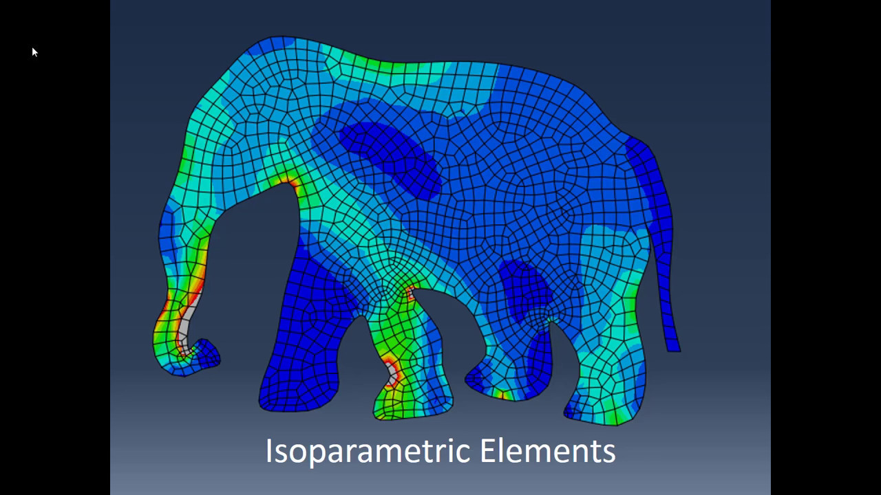
FEA 26: Isoparametric Elements
Contoh Perhitungan Analisa Balok Anak dgn Plastik Sempurna (Leleh Umum) | Struktur Baja | Lightboard
Beban Terfaktor (Ultimate Load) dan Kuat Rencana (Design Strength) Struktur Baja | Lightboard
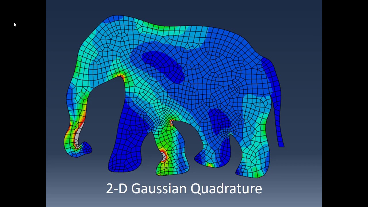
FEA 30: 2-D Gaussian Quadrature
Belajar SAP2000 Pemula (Bagian ke-1 Balok Sederhana)
SAFE - 08 Cracked Section Analysis: Watch & Learn
5.0 / 5 (0 votes)
