W6L1_Union Find Data Structure

Summary

The video script delves into the intricacies of Kruskal's algorithm for finding minimum cost spanning trees, emphasizing the role of the Union-Find data structure. It explains the initial naive implementation of Union-Find, where union operations are costly. The script then introduces an optimized approach using two dictionaries to track components and their sizes, allowing unions to be performed more efficiently. The concept of merging smaller components into larger ones to reduce the complexity of union operations is highlighted. The summary also touches on the amortized analysis that proves the improved union operation's efficiency, ultimately enhancing Kruskal's algorithm's performance to near-linear time complexity.

Takeaways

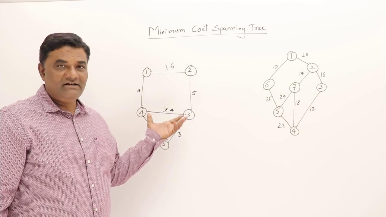
• 🌳 The script discusses two algorithms for finding minimum cost spanning trees: Prim's and Kruskal's algorithms.
• 🔍 Prim's algorithm extends a tree by finding the shortest edge connected to the current tree, similar to Dijkstra's algorithm.
• 🌉 Kruskal's algorithm builds a tree by starting with disconnected nodes and adding the shortest edge possible without forming a cycle.
• 🔢 Kruskal's algorithm involves sorting all edges in ascending order and then processing them to build the minimum cost spanning tree.
• 🔄 A key challenge in Kruskal's algorithm is efficiently tracking the components (sets of connected vertices) as edges are added.
• 🔑 The 'find' operation identifies the component a vertex belongs to, while the 'union' operation merges two components into one.
• 📈 Initially, union operations can be inefficient, taking O(n) time, as they require updating all vertices in the smaller component.
• 📚 The script introduces a data structure to improve union find operations, using dictionaries to track components and their members.
• 🔑 By keeping track of component sizes and merging smaller components into larger ones, the union operation can be optimized.
• 📊 The amortized complexity of the improved union find is O(log m) per operation, leading to significant efficiency gains in Kruskal's algorithm.
• 📈 The overall time complexity of Kruskal's algorithm, with the optimized union find, becomes O(n log n), a substantial improvement from the naive O(n^2).

Q & A

What are the two algorithms mentioned for finding minimum cost spanning trees?

The two algorithms mentioned for finding minimum cost spanning trees are Prim's algorithm and Kruskal's algorithm.

How does Prim's algorithm extend a tree in the context of minimum cost spanning trees?

Prim's algorithm extends a tree by finding the shortest edge connected to the current tree.

What is the initial state of nodes in Kruskal's algorithm?

In Kruskal's algorithm, the initial state of nodes is disconnected.

How does Kruskal's algorithm build a minimum cost spanning tree?

Kruskal's algorithm builds a minimum cost spanning tree by starting with disconnected nodes and connecting them by adding the shortest edge possible, processed in ascending order.

What is the main difficulty in implementing Kruskal's algorithm efficiently?

The main difficulty in implementing Kruskal's algorithm efficiently is keeping track of the components and determining which nodes belong to the same component or different components as edges are added.

What is the purpose of the 'find' operation in the context of Kruskal's algorithm?

The 'find' operation is used to determine which partition a given vertex belongs to, which is crucial for checking if adding an edge would form a cycle.

What does the 'union' operation in Kruskal's algorithm achieve?

The 'union' operation in Kruskal's algorithm merges two components into a single partition when an edge connecting them is added to the spanning tree.

Why is the 'union' operation considered time-consuming in the initial implementation of Kruskal's algorithm?

The 'union' operation is considered time-consuming because it requires finding all other vertices in the same component as a given vertex and updating their partition, which involves a linear scan proportional to the size of the set.

How can the efficiency of the 'union' operation be improved in Kruskal's algorithm?

The efficiency of the 'union' operation can be improved by keeping track of the size of each component and always merging the smaller component into the larger one, which reduces the number of elements that need to be relabeled in each operation.

What is the amortized complexity of the 'union' operation in the optimized version of Kruskal's algorithm?

The amortized complexity of the 'union' operation in the optimized version of Kruskal's algorithm is O(log m), where m is the number of union operations.

How does the optimized union-find data structure contribute to the overall efficiency of Kruskal's algorithm?

The optimized union-find data structure contributes to the overall efficiency of Kruskal's algorithm by reducing the time complexity of the 'union' operation, which in turn brings the overall time complexity of the algorithm down from O(n^2) to O(n log n).

Outlines

00:00

🌳 Introduction to Kruskal's Algorithm and Union-Find

This paragraph introduces Kruskal's algorithm for finding a minimum cost spanning tree, contrasting it with Prim's algorithm. It explains that Kruskal's builds the tree from the ground up by adding the shortest available edges without forming cycles. The challenge lies in efficiently tracking the components (sets of connected vertices) as edges are added. The paragraph outlines the need for 'find' and 'union' operations within a disjoint set data structure to manage these components, highlighting the inefficiency of naive union-find implementations due to the need to update all elements in a component.

05:05

🔍 Inefficiency of Naive Union-Find and the Need for Improvement

The second paragraph delves into the inefficiency of the naive union-find method used in Kruskal's algorithm. It describes how the union operation, which combines components, requires a full scan of all elements to update their component assignments. This results in an O(n) time complexity for each union, which becomes a bottleneck when performing multiple unions. The paragraph emphasizes the need for a more efficient data structure to handle the dynamic nature of component updates during the algorithm's execution.

10:09

🔄 Enhancing Union-Find with Component Tracking

The third paragraph introduces an enhanced union-find method to improve the efficiency of Kruskal's algorithm. It discusses the use of a 'members' dictionary to track which vertices belong to which components and a 'size' dictionary to keep count of the vertices in each component. This allows the union operation to be more efficient by only iterating over the vertices in the smaller component, rather than scanning all vertices. The paragraph outlines the updated union and find operations and explains how this approach reduces the time complexity of union operations.

15:13

📈 Amortized Analysis of the Improved Union-Find

This paragraph provides an amortized analysis of the improved union-find method. It explains that by always merging the smaller component into the larger one, the size of any component grows exponentially with each union operation. Since the largest component can only be as large as 2m (where m is the number of union operations), the number of times a component can double in size is limited to log m. This insight leads to the conclusion that the amortized time complexity of a union operation is log m, significantly improving the overall performance of Kruskal's algorithm.

20:18

🔗 Impact of Improved Union-Find on Kruskal's Algorithm

The fifth paragraph discusses how the improved union-find method impacts the overall time complexity of Kruskal's algorithm. With the new method, the sorting of edges takes O(m log m) time, and the union operations, which are performed n-1 times (where n is the number of vertices), take O(n log n) time in total. The paragraph concludes that the overall time complexity of Kruskal's algorithm is now O(N log N), where N represents the size of the graph, a substantial improvement over the naive implementation.

25:21

🌐 Advanced Union-Find Techniques and Their Impact

The final paragraph explores advanced techniques for the union-find data structure, such as using trees to represent components and applying path compression to flatten these trees. This approach can reduce the time complexity of both union and find operations to almost constant time, further optimizing Kruskal's algorithm. The paragraph encourages further exploration of these advanced techniques for their potential to make each union-find operation cost-effective.

Keywords

💡Minimum Cost Spanning Trees

Minimum Cost Spanning Trees (MCST) are a theme central to the video. They are a subset of the edges of a connected, undirected graph that connects all the vertices together, without any cycles and with the minimum possible total edge weight. The video discusses two algorithms for finding MCSTs: Prim's and Kruskal's. Prim's algorithm starts from a single vertex and grows the tree one vertex at a time, while Kruskal's algorithm starts with all vertices as separate trees and merges them incrementally using the smallest available edge that doesn't form a cycle.

💡Prim's Algorithm

Prim's Algorithm is a greedy algorithm used to find the minimum spanning tree in a connected, undirected graph. It is mentioned in the script as the first algorithm studied for MCSTs. It works by starting with an arbitrary node and at each step, adds the cheapest edge that connects a vertex not yet in the tree to the tree.

💡Dijkstra's Algorithm

Dijkstra's Algorithm is a graph search algorithm that solves the single-source shortest path problem for a graph with non-negative edge weights, and it is referenced in the script in comparison to Prim's algorithm. Although not directly about minimum spanning trees, it shares the 'greedy' nature of Prim's in extending a solution incrementally by the shortest edge.

💡Kruskal's Algorithm

Kruskal's Algorithm is another algorithm for finding the minimum spanning tree, which is discussed extensively in the script. It is a 'bottom-up' approach that starts with all nodes as separate and progressively merges the lightest edges that do not form a cycle, eventually forming a single tree that spans all nodes.

💡Disjoint Sets

Disjoint sets are sets that do not have any elements in common. In the context of the video, disjoint sets are used to represent the collection of components in Kruskal's algorithm before they are merged to form the minimum spanning tree. The script discusses how to keep track of these disjoint sets efficiently using union-find data structures.

💡Union-Find

Union-Find, also known as Disjoint Set Union (DSU), is a data structure that keeps track of a set of elements partitioned into multiple disjoint subsets. It is crucial to Kruskal's algorithm as it helps to determine whether adding an edge would form a cycle. The script describes how to implement union-find with efficient operations for 'find' and 'union'.

💡Find Operation

The 'find' operation in union-find is used to determine which subset a particular element is in. The script explains how this operation is implemented in the context of Kruskal's algorithm to check if two vertices are in the same subset, which would mean adding the edge would form a cycle.

💡Union Operation

The 'union' operation in union-find is used to merge two subsets into a single subset. In the script, it is described as a critical operation in Kruskal's algorithm, where it is used to join two components into one when the corresponding edge is added to the minimum spanning tree.

💡Path Compression

Path Compression is an optimization technique used in union-find data structures to flatten the structure of the sets, reducing the cost of 'find' operations. It's mentioned in the script as a technique that can be applied to make the 'find' operation almost constant time, thus improving the efficiency of the algorithm.

💡Amortized Analysis

Amortized Analysis is a method to analyze the average time complexity of an algorithm over a sequence of operations, considering the worst-case scenario for individual operations might not reflect the overall performance. The script uses amortized analysis to argue that the 'union' operation in the improved union-find has an amortized time complexity of O(log m), which is crucial for the efficiency of Kruskal's algorithm.

💡Sorting

Sorting is a fundamental algorithmic process discussed in the script, specifically in relation to the initial step of Kruskal's algorithm where all edges are sorted by weight. The efficiency of sorting affects the overall time complexity of the algorithm, with the script noting that sorting takes O(m log m) time.

Highlights

Introduction to minimum cost spanning trees and algorithms like Prim's and Kruskal's.

Explanation of Prim's algorithm and its approach to extending a tree by finding the shortest edge.

Description of Kruskal's algorithm and its method of building a tree bottom-up by adding the shortest edges.

The importance of sorting edges in Kruskal's algorithm and the process of adding edges without forming cycles.

Challenge of tracking components in Kruskal's algorithm and the need for efficient data structures.

Introduction to the concept of disjoint sets and their role in Kruskal's algorithm.

The function 'find' and its role in determining the partition a vertex belongs to.

Explanation of the 'union' operation and its impact on merging components.

Discussion on the inefficiency of the naive union-find implementation in terms of time complexity.

Introduction of the improved union-find data structure with 'members' and 'size' dictionaries.

Optimization of the 'union' operation by merging smaller components into larger ones.

Analysis of the amortized complexity of the improved union-find algorithm.

Explanation of how the improved union-find affects the efficiency of Kruskal's algorithm.

Final time complexity analysis of Kruskal's algorithm using the optimized union-find data structure.

Introduction to path compression and its role in further optimizing union-find operations.

Conclusion on the overall improvement of Kruskal's algorithm through the use of advanced union-find techniques.

Transcripts

When we studied minimum cost spanning trees, we saw two algorithms. The first one was Prims

algorithm, which, like Dykstra s algorithm, tried to extend a tree by finding the shortest

edge connected to the current tree. And the other was Kruskal s algorithm.

So, in Kruskal s algorithm, we built up a tree bottom up. We started with disconnected

nodes, and then we connected them by adding the shortest edge possible. So, we begin by

processing all the edges in ascending order, of course. So, we sort the edges, you pick

up the smallest edge, and each time we pick up an edge, we see if the edge forms a cycle.

So, we have a collection of components, which have already been joined together by the edges.

And if the new edge does not create a cycle within a component, we add it. And in the

process, what happens is that the endpoints of the edge u and v belonged earlier to different

components. Because if they were in the same component, the component is connected, it

would form a cycle. But having now connected these two components together, we must merge

the components as we go along, so that we do not add another edge within this component.

So, the main difficulty that we saw with implementing Kruskal s algorithm efficiently was precisely

this task of keeping track of where the components were at any given time. So, we know that in

the beginning, it is all disjoint because it is a bottom up algorithm, everything is

a singleton. But as we go along and edges are added, which edges are, which nodes are

part of the same component, which ones are different components, this was the problem.

So, abstractly, what we have is a collection of vertices, which are partitioned. So, this

is a collection of disjoint sets, every vertex belongs to one of the partitions. And no vertex

belongs to two partitions. So, the collection of partitions together gives us the full set.

But each collection in that partition is in, is in, has an empty intersection with every

other collection. And now given this partition, so, we have this kind of picture that we have

a set.

And it has now been divided like this, into these disjoint partitions. And now I say,

I give you a vertex u and I asked which partition it belongs to? So, that is, this expression,

this function called find. So, find tells us which partition a given vertex belongs

to. And similarly, now when I take say u belongs to this, and say v belongs to this, then after

this edge has been added. So, I have now found an edge which connects u and v.

Now, these two become the same partition. So, I have to have a second operation, which

says given two elements of the set of the collection with the set I am dealing with,

take their partitions and make them into a single partition. So, the union operation

and the find operation and what we actually saw in Kruskal s algorithm was this, this

union operation is what took us time. Because we had to find all the other vertices which

are in the same collection as u, same partition as u and convert them to the same partition

as v.

So, what we need is a data structure, which can implement these operations. So, essentially

we have a set, a set of elements which is partitioned into components. So, as we said,

partition means that C1 union C2 union Ck is actually all of S. And each element, small

s in S belongs to exactly one of the Cis or Cjs. So, this is what it means to be a partition.

And now, we need to first create the initial partition.

So, the initial partition is going to be the one where every element is on its own. So,

you have a singleton partition containing just s for every small s, in your set. And

then we have these two operations as we said, find and union. So, find tells us the name

of the partition or the name of the component that s belongs to. And union given two set

elements, s and s prime tells us, gives us back a single component for all the elements

in the same component as s and s prime together.

So, let us for simplicity assume that our elements are numbered 0 to n minus 1, this

is what we typically do even for vertices when we deal with graphs. We deal it, we will

typically use 0 to n minus 1 as the names of our vertex set. So, we will set up a mechanism

to keep track of the components and the easiest way is to have either a list or an array or

a dictionary, where now because these are 0 to n minus 1, I can interpret these as indices

in the list or as keys in the dictionary or as positions in the array.

So, if I look up the eighth element of component, it will tell me which component the element

i belongs to. So, now what does make union find do? Make union find basically creates

names for the components, which are the same as the vertices. So, I have, I have elements

0 to n minus 1 and I also have components. So, this is just for convenience, I do not

want to create another set of names. So, the components are also called 0 to n minus 1.

So, 0 goes to component 0, 1 goes to component 1, and so on. Because I need a name for the

set. The component containing 7, the component containing 6, so I need a name for that set.

And those names are going to be just the same 0 to n minus 1. So, component of the element,

i will be the component i, that is what this is saying, component of the element i. So,

this is the element, and this is the component number.

This is how we set up our thing and make with this make union find. So, we have this, say,

dictionary component. And now when I want to find out which component vertex i belongs

to or a set element i belongs to, I just query this dictionary, I will look at probate with

the index, or the key value i. And the, what is stored in the dictionary is the component

number. So, initially, it is i and it will change as it goes along because of unions.

So, let us see how union works. So union, as we saw is basically a sequential scan.

So, you want to now take two elements, i and j, and combine their components. So, over

time, they have reached some component name. So, if I look at component of i, it is some

c old and c new because I am going to merge in this, I am assuming that I am going to

put everything which is in component of i into the same component as j.

So, I am not going to change the names of the component for the same component as j,

I am going to change the name of the component for things which belong to the component of

i. So, let us say component of i is old component c, and component of j is a new component c

new. Now, I have to take every vertex, and this is the part that is inefficient. I have

no idea which other nodes have the same component as i.

So, I have to take every other vertex. And if that vertex has a component, which is the

same as i, I will reset its component to be the same as j. So, this is once linear scan,

which is proportional to the size of the set, which I have to do every time I do a union.

It does not really matter whether the component of i was small or not. I have to look at every

other vertex because I have no indirect information about which other vertices have been merged

with i, so far.

So, what is the component of i contain? So, with this, it is easy to see that this make

union find takes order n. Because I have to go through and label the component number

as i for every vertex i. So, this is just a simple linear scan across all the elements

in my set. Find just looks up a dictionary. So, if we assume that this is a dictionary,

or an array with a constant time lookup of the ith element, then in constant time, or

O, one time, I will find the component for a given element i.

But union as we can see, takes time proportional to the size of the set. Because I have to

go through every element in the set and check if it has got to be merged or not. Whether

or not it has to be merged, I have to check it. So, this is much like an adjacency matrix

representation of a graph, in order to find the neighbors of a vertex, you have to scan

all the columns whether or not this vertex has few neighbors, or has many neighbors,

you have to scan all the columns to find the neighbor.

So, in the same sense, you have no idea how many elements share a component with i, so

you have to scan all of them. And wherever you find something which shares a component

with i, you have to move it to j. So, this means that one union operation takes order

n time. So, if I give m union operations, then it is going to take m times n time. So,

this is going to be the bottleneck that we saw.

Because in Kruskal s algorithm, we have to add n edges or n minus 1 edges to make a spanning

tree. So, we do order n merges, and naively speaking, if we do order n merges and each

merge takes order n time, then I spent order n squared time executing all of Kruskal s

algorithm. And that is what we are trying to improve.

So, how do we improve this? Well, what is the bottleneck? So, the bottleneck is that

we do not know, so if I am sitting here and if I have a component which contains i, I

do not know what are the other vertices in this component. So, this whole component has

some name c. So, I know that component of i, is C. The question is what other vertices

have components c. So, which are the other vertices in the same component?

So, now we keep track of an int, an dictionary going the other way. So, component tells us

given a vertex, which component it belongs to. Members tells us given a component, which

are the vertices which belong to it. So, members of c will be list, it will give you a list

of vertices. In general initially, for example, I will have members of, of the ith component

will just be the list i. Because, initially every component has only one vertex, but as

it grows, it will be a longer list.

And of course, now since this is a list, I can take its length. I can take the length

of this members c, and I will know how many vertices belong to this component. But I do

not want to actually spend time computing the length each time. So, I will separately

store this as size of c. So, I am keeping track of two new dictionaries. One is members

of c, members of c says give me a component and give me the list of vertices belong to

this component.

Size of c says, how many vertices are there, which is just the length of that list. But

I do not want to compute that list explicitly each time, so I will just keep track of it

because it is easy to update as we will see. Now given this, let us see how to do our implementation.

So, first we have to implement this make union find initial step, where we create the singletons.

So, we had this old step which we repeat, which is we for every vertex for every element

i.

I set the component of i to be the actual component i itself. So, remember that we were

using i for both 0 to n minus 1 to name both the elements and the components. So, the component

of i is just a component i. On the other hand, we have to now do the reverse map. So, we

have to say what does component of i contain? Well members of i is the list containing i.

And size of component i is 1. Because I have only singleton's at all point. So, this is

the initialization, very straightforward.

What about find? Well, find does not update anything, find very looks up the component.

So, it does not have to look at members or size because it just needs inform, information

in the dictionary component. So, as before find of i just looks up component of i. Union

is where we were having problems, so let us see if we can make union a little more efficient.

So, as before, we find out the names of the components of the two vertices are two elements

we are dealing with i and j.

So, we are going to as before, assume that we are moving everything in the component

of i, to be in the component of j. So, we call the component of i as c old and the component

of j as c new. And this difference now is that instead of going over everything, before

we were doing this for loop over every element in our set, for every vertex in our set. So,

we are going from 0 to n minus 1. But now I do not have to do it for every vertex, (())(12:30)I

know which ones have to change.

The ones that have to change are the ones that are in the same component as i. So, I

just have to look at the list members of c old and for every k members of c old, I will

first of all change its component. I will update its component from c old to c new.

But now I have to keep track of these other things as I go along. So, I have to take this

c new component and append this new element to its list. So, a k is now being added as

a new element in members of c new.

So, as I change the name of the component of k from c old to c new, I go to the members

of C new and I add k to it. And when I add k to it, its size also changes. So, I also

increment the size of c new by 1. So, these are two extra steps, which happened when I

re label, when I move vertex from this component to that component I must add it to its list

members and I must upgrade the size by 1. So, this is simple enough.

So, the question is what have we gained? Because what we have gained really is this step. Compared

to our earlier implementation, this is still order n and this is still order one. So, the

question is what have we gained in union? So, the point is that by going over members

of c old we can get away with only working with this many elements rather than this many

elements. So, when I re label instead of looking at order n elements, I am looking at order

of the size of the component.

So, this is similar to our graph theoretic things where we say that when we look at the

neighbors of a vertex, we are interested in the degree of the vertex, the actual edges

rather than all the neighbors which are not (())(14:14). So, in the same spirit, we are

only interested in those elements which belong to this component. We are not interested in

scanning all the components, so we are explicitly keeping that in this members list.

So, the question is so, this is fine, we are using members here. But why are we keeping

track of the size? Because there is no apparent reason in this whole thing except that we

have to update it correctly and all that. Nowhere are we using size in this union operation.

We are just updating it. We are updating it for sure, but we are not using the fact that

the size is available to us. So the way we will use size as follows.

We will always choose whether to, so we remember we have a choice. We can either go from i

to j or j to I, which component gets relabeled as which component. Do I make everything in

come opponent of i point to j or make everything and component of j point to i. So, that is

where size will play a role. So, size will say that we only always merge the smaller

component into the bigger component.

So, we have basically two components. So, if i belongs to c and j belongs to c prime,

I have to decide whether to make everything in c the same as c primer, or everything in

c prime. So, the final component that survives is going to be c or c prime? So, the rule

is that the larger component will survive. So, if c is smaller than c prime, I will rename,

re label everything reliable everything inside c to be c prime.

And if c prime happens to be smaller than c, I will do the opposite. So, that is the

crucial decision that size gives us. So, a priori does, does not seem to be so helpful.

Remember, our problem was that when we were doing this as range of n, blindly, we were

spending order n time on every merge. But now we are spending something proportional

to the size of the smaller set. But the size of the smaller set could still be almost half.

It could be half plus a little bit, half minus a little bit. So, in the worst case, a single

merge operation could still be order n. Because it could be taken by two steps. So, we have

not really guaranteed that an individual merge operation is less expensive now, up to an

order constant factor. Of course, it will be half as expensive, but half is not good

enough. It is a constant factor, we want something which is a little more strong than half.

So, it turns out that this we cannot deny, I mean, it could be that an individual merge

will cost half n time. But it will not happen frequently. So, we have to do our accounting

a little carefully. So, we are not going to change the implementation. This is our final

implementation. But we are going to argue that this is good enough, when we have this

rule, of always merging the smaller component to the larger component, we are actually going

to get a sizable improvement.

So, why does this happen? Well, basically, if I take a vertex i and I track what happens

to i. So, initially, its component is i. The first time it is forced to change its component,

it changes its component from some c to c prime. Then from c prime to c double prime.

But what I have guaranteed now is that when I take i and I look at the component it belongs

to and Now supposing this is the other component, which has j and I now merge this.

Then i moves from c to c prime, but c prime was at least as big as c. Because c prime

was a bigger component. So, if c had some k elements, then c prime has more than k elements.

So, totally now, the component of i has gone from k to something bigger than 2k. So, the

size of the component of i doubles every time it is labeled. So basically, each time I re

label the component of i, I move it to a set, which is twice as big as it was before, at

least twice as big, could we could be even bigger.

Now the other point to note is that when I do a merge, how many different elements change

their component from the initial state. So, initially, remember, I have 0 to n minus 1,

as components, 0 to n minus 1. Now at some point, I do a merge. So, maybe I take i and

j. So, I take these, and then they will both go say to j. So, at this point, I have touched

i and j. So, I have changed their component structure. In the case of one I have changed

the component name and the other one, I have changed it to be in a component, which has

new elements.

Now the question is, after m such things, after m union operations, how many elements

have had their component touched in this way, either it has moved, or something has come

into it? Well, you can see that, if I take two elements, then I had touched two. The

next merge could, next union could take two other elements and touch two. So, I could

do 2 plus 2 plus 2, which is 2. The first merge, first union merges these two, next

union merges these two.

But I cannot do any more than that, I claim. Because if I do not take two new elements,

then I must be taking some set which has already been touched and one more element. So, at

most, I can touch 2m elements. So, this means that at most 2m elements have had their component

updated since the beginning. But if at most 2m elements have had their components updated,

the worst that can happen is that all of them are merged into a single component.

I cannot have a larger component than that. So, the largest component of any vertex in

my set is at most 2 times m. So, many of them will still have singletons, this is what we

are saying. So, after m union find, m union operations, the largest set in my partition

cannot be bigger than 2m. So, we have now these two facts. The fact is that each time

I change the partition of i, it moves to a set, which is twice as big.

But it cannot go beyond a certain size because across m operations, it can only grow up to

2m. So, combining this, we see that the size of a component will grow from 1 to 2 to 4

to 8, but it has to stop before 2m. Because it cannot get beyond 2m, because 2m is the

largest set I could possibly have, after m union operations. So, that means is doubling

can happen at most log m times.

That means if I pick a vertex, and I examine how many times it changes its component, it

can be at most log m times. So, a single vertex cannot change its component more than log

m times. So, this is what gives us now a better bound for union find.

Because it says that basically over m updates. First of all, we know that at most, 2m elements

are relabeled. And each of them is relabeled at most log m times. So, the remember our

relabeling operation is now optimal, I never look at a vertex to re label unless I need

to. Because I am looking only at members of c. So, every time I did decide whether to

re label a vertex or not, I am going to re label it, I never look at a vertex and, and

do not re label it.

So, if I only need to know how many reliable operations are there, because I never look

at vertices, or try to do anything with vertices in union when I am not relabeling them. But

I know that a, there are at most 2m of them, because that is the limit of how many vertices

ever get relabeled. And each one of them gets done at most log m times. So, if I add it

up, it is like, again, it is a similar analysis. But in a more complicated setting.

When we said that, when you do breadth first search or depth first search using an adjacency

list, then as we process all the vertices, we do the sum of the degrees. So, an individual

vertex might add a lot of neighbors to the queue in breadth first search but others will

add less. And totally the number of neighbors I have to look at is going to be the sum of

the degrees and therefore it gets bounded by the total number of edges.

Similarly, here, we are saying that the total number of operations of relabeling across

all the M union operations is going to be m times log m. Because 2m, order of m times

log m, let us say. Because 2m vertices are going to get elements are going to have the

labels change, and no element is going to be touched more than log m times. So, therefore,

over m union operations, I will not do more than m times log m work, in terms of changing

component numbers.

So, this is where we have saved. So, instead of going to m times n, we have come to m times

log n. So, this means that if I have, since I am assuming that there are m of them, I

can take m times log m. And I can say what is the cost of one of them? I divide it by

m. So, on an average, in a sense, each of them is only taking logarithmic time. So,

it is not that any one of them is actually taking logarithmic time for sure.

Because I know that sometimes I have to merge a large component. But then many of the times

I will be merging very small components. And if I add it up, so this is again, this notion

that we saw with, as I said, with BFS and DFS, when we were dealing with adjacency lists,

that we count the cost across the entire operation and say the total sum of the operation can

only be so much. Even though individual, individual operations can be more.

So, this is, this notion of amortized, what you gain in one place, you will lose in another

place. But overall, it will all work out. So, the amortized complexity of one union

operation is log m. Even though individual union operations could be more expensive,

totally m log m is the cost of m such operations.

So, how does this affect Kruskal s algorithm? So, this is where we started looking at these

operations, because this was the context in which we needed it. So, remember that, in

Kruskal s algorithm, we start by sorting the edges. So, we take the edges, there are m

of them, and we sort them in ascending order. After this, we have to start this business

of creating the tree. So, we have to keep track of these components.

So, we first do a make union find, which will take order n time for our n vertices. So,

this is going to be ordered n time. Now, when I check whether a vertex needs to be added

or not, I need to look up the component name of the two endpoints. But this is order 1

time because I just have to look up my component (())(24:27). And now this is the step which

was bothering us. So, earlier this was taking order n time when we did it naively.

But now we know in this amortize sense is going to take log m time. So, how many union

operations are we going to actually perform? Well, because they are constructing a spanning

tree on n vertices and a spanning tree on n vertices remember will have n minus 1 edges

exactly. We are going to do exactly n minus 1 union operation. So, we can think of it

as the order n union operations. So, we saw earlier that if we do order m, if you do m

operations is m log n.

So, here it is n operation, so it is n log n. So, the total cost of all these union operations

across each addition that we actually perform, remember that if find u turns out to be find

v we just throw away the edge, so we do not do anything. So, only when find u is not equal

to find v, when they are in two different components, we have to do a merge. But now

what we are saying is that this merge, will actually happen overall, the overall cost

of these merges, they will be n of them will be n log n.

So, this is the amortized cost over all of the union operations. So, now, if we go back

to the first step, this is another expensive step. This takes m log m time using an optimal

sorting algorithm. So, we have, we have seen that, things like merge sort, for instance,

are m log m. And a naive algorithm like insertion sort of selection sort could be n squared.

But you cannot beat m log m, we said without giving a proof saying that that is a lower

bound.

So, we need to spend m log m time to sort. So, we need m log m time to sort and n log

n time to do the unions. Now, this is kind of bit awkward to have log m here and log

n there. But notice that m is at most n squared. So, if I take logs on both sides, I will say

log m is less than equal to 2 of log n. So, this is how logs work. So, log of m is actually

big O of log of n, it is some constant times log of n.

So, I can say that m log m is the same as m log n. So, now I have the same thing on

both sides. Now, I am in good shape, I have n log n and I have m log n.

So, I can now combine them and claim that the overall time of Kruskal s algorithm is

m plus n times log n. So, remember that this really is the size of of G. So, we are really

saying that in terms of the size of G, it is N log N. I mean, if you think of capital

N as the size of G, it is within capital N log N.

And this is probably the best that one could hope to do given that you have to do sorting

and all that. So, this is how this union find algorithm actually helps us bring Kruskal

s algorithm down from n squared to something like n log n.

So, what we have seen is that if we use this two way mapping, so component is the obvious

thing. It tells us given an element which component it belongs to. But if we keep the

reverse mapping, given a component, which are the elements which belong to it, then

we can relabeled these components efficiently by also keeping track of the size, always

merge a smaller component into a bigger component.

And if we just follow this rule of merging smaller components into bigger components

and keep track of the components using this member array, then or member dictionary, then

we can guarantee that across m operations, the amortized complexity of each union operation

is log m. So, m log m is the total cost of all the unions, find remains constant time

because it is just looking up a dictionary value.

And make union find remains linear time because I have to actually reset the component to

a singleton for everybody. So, this is a very direct and easy way of doing union find, there

is a slightly more complicated way where instead of keeping this members of k as a list of

vertices, you can keep it as a tree. And if we keep it as a tree, then it turns out that

union operation becomes very simple. So, basically, I will have members of i. So, this will be

some tree. And I will have members of say j and this will be some other tree.

And the rule is that if you belong to the same tree or the same component, so the union

operation will just either connect this tree that way, or connect this tree this way, so

it will just take the root of one tree and put it as a child of the root of the other

tree. So, the union operation is very simple, I just stick one tree under the other tree.

But now find means, I am sitting here and I must go up to the root, the root vertex

will tell me which component I am in.

So, we have to be careful that these components, these trees do not become very tall. And there

is a clever way of keeping them not only from growing very tall, but actually flattening

them. There is something called path compression that you can do. And if you do this path compression,

eventually your tree will look like this, where everything so if I have a component

and I have all the other vertices which belong to the component will be only one step below.

So, it will only take me one lookup in order to tell you what component is. So, it will

have an amortized complexity of almost constant time. So, both union and find become so union

is constant and find is almost constant. So, this is really the ultimate implementation

that you could have for this where you can keep track of this and then each operation

is a unit cost. But we will not go into that now. But you can look it up. It is a very

interesting optimization of this union find data structure.