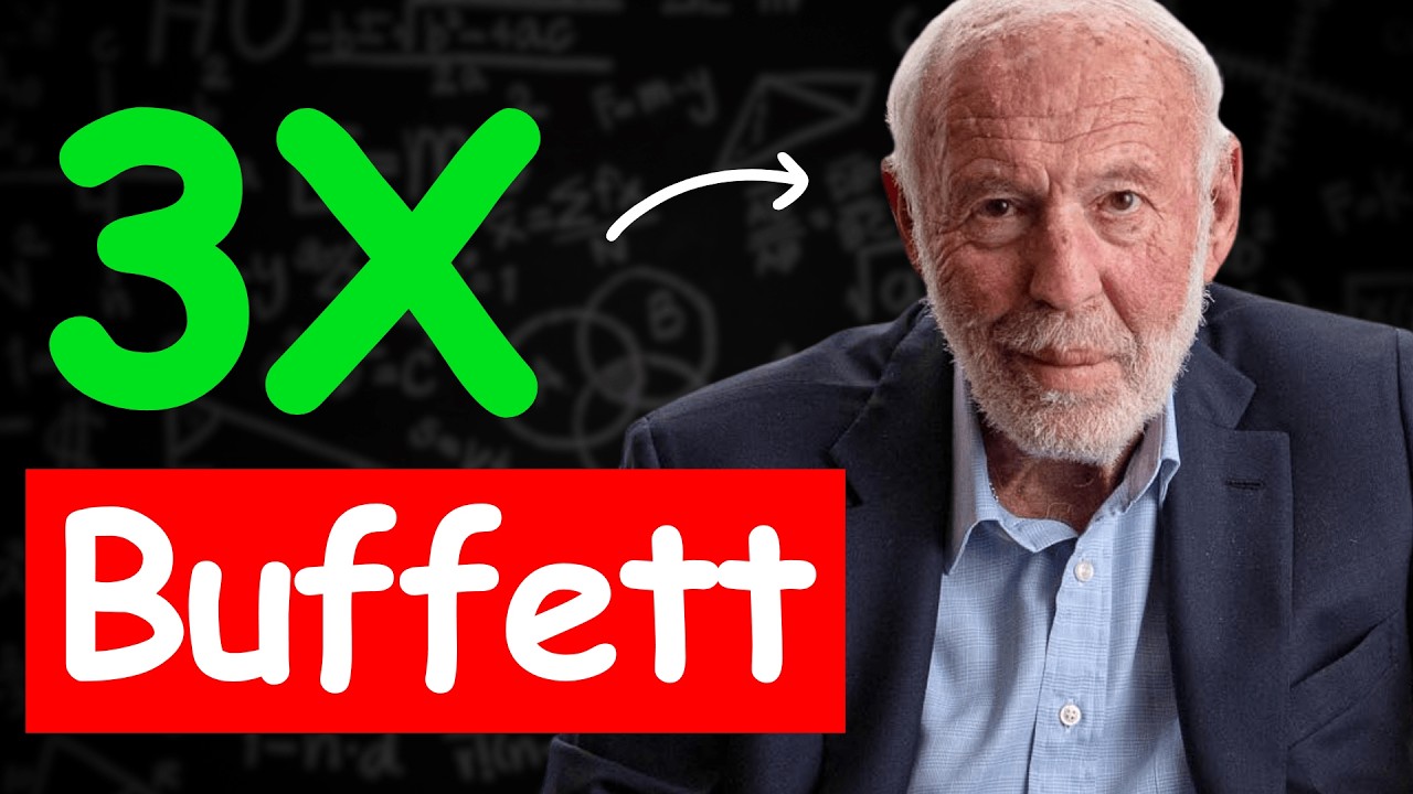
Jim Simons Trading Secrets 1.1 MARKOV Process

Summary

The provided video script explores various quants and trading strategies inspired by Jim Simons' secretive quant fund Medallion which have achieved high returns. It delves into concepts like Markov processes, mean reverting strategies, and backtesting approaches used by simons to assess probabilities and performance, coded in Python. The speaker analyzes a specific mean reverting strategy Q5 from his course, evidencing its effectiveness across various recession periods. He conveys how quants leverage data, tools and skills to calculate probabilities favoring their trading strategies.

Takeaways

• 😀 Jim Simons' Medallion fund has averaged 39% annual returns over 30 years, proving Quant strategies can work very profitably over the long term
• 😮 Key people like Ax and Lofa worked for Simons, developing advanced mathematical models like Markov chains to predict markets
• 📈 Recessionary periods see very high volatility which suits mean reverting Quant strategies extremely well, leading to huge returns
• 📊 The Markov chain method models random sequences of market events where future probabilities depend only on the current state
• 😃 A simple example is modelling a 'Markov' person who randomly visits home, shop and work with differing probabilities
• 🤔 These probabilities can be encoded in a 'transition matrix' to represent the likelihoods between market states
• 📉 Using Python we downloaded S&P500 data, calculated up/down days, and derived the probability matrix for consecutive days
• ✅ The best probability was a 57% chance of an up day following 5-6 down days - this simple rule gave 46% 10 year returns
• 🎯 Multiple Markov model conditions can be combined across stocks and strategies to improve performance and reduce drawdowns
• 🌟 The key is using data, tools and skills to systematically turn market probabilities in your favor - as Quants like Simons do

Q & A

What is a Markov process in quantitative trading?

A Markov process in quantitative trading is a random sequence of market events or price changes where the probability of future events is based only on the current state of the market, not on past states.

How did the mean reverting strategy perform during recessions according to the transcript?

The transcript states that the mean reverting strategy performed extremely well during the 2008 recession, the 2001-2002 recession, and the recent 2022 recession, significantly outperforming the broader market.

What is an example of a transition matrix in the Markov model?

An example transition matrix shows the probabilities of an up day following an up day (0.54), a down day following an up day (0.45), an up day following a down day (0.57), and a down day following a down day (0.42).

What Markov model probability was most significant in the transcript?

The transcript showed that the probability of an up day following 5-6 consecutive down days was 66%, which was considered a significant probability to trade on.

How can the Markov model be enhanced according to the video?

The video suggests enhancing the Markov model by adding more conditions, applying it to multiple stocks, using machine learning to calculate probabilities, and utilizing a for loop to test different combinations.

What Python libraries are used in the Markov coding example?

The Python coding example uses the pandas, NumPy, and yfinance libraries to download the data, calculate the probabilities, and create the transition matrix.

Who is Jim Simons and what is significant about him?

Jim Simons is considered one of the greatest quant traders of all time, running the very successful Medallion fund for decades using quantitative strategies, which has massively outperformed traditional investors like Warren Buffett.

What is the benefit of using Markov models in trading?

Using Markov models can help traders objectively calculate probability statistics to determine high-probability trading opportunities with an edge over randomness.

What were some key strategies used by Medallion fund quants according to the transcript?

The transcript mentions Medallion fund quants using mean reversion strategies based on the idea that prices tend to revert after an initial move up or down, as well as Markov chain models.

What Python library allows easy backtesting of trading strategies?

The transcript demonstrates using the Pine Script editor to easily backtest and visualize trading strategies in Python before deploying them live.

Outlines

00:00

Introducing Markov Chains and Transition Matrices

This paragraph introduces the concept of Markov chains, explaining that they are random sequences of events where the probability of future events depends only on the current state. It provides a simple example comparing a human going from home to shop to work, versus a 'Markov' whose next move depends only on his current location. The paragraph then explains how transition matrices capture the probabilities of different sequences of events in a Markov chain.

05:01

Illustrating Markov Chains for Trading

This paragraph provides a trading example for Markov chains and transition matrices. It shows hypothetical positive/negative percentage moves for a security, and the probabilities of a positive or negative move the next day. These probabilities are arranged in a transition matrix showing the likelihoods of different sequences of up and down moves.

10:04

Building a Markov Model for S&P500 Trading

This paragraph walks through Python code to build a Markov model for S&P500 trading. It calculates the actual probabilities of sequences of positive and negative return days in S&P500 data from 2010-2022. The code prints out a transition matrix showing the probabilities of different combinations of up and down days.

15:06

Using Markov Models to Create Trading Strategies

This paragraph explains how the Markov probabilities can be used to create effective trading strategies. It shows a simple strategy based on a 66% chance of an up day after 5 down days, backtested in Pine editor. It emphasizes combining multiple conditions and strategies to further improve performance, as likely done in the Medallion fund.

20:08

Conclusion and Invitation for Questions

The final paragraph concludes by summarizing the goal of explaining Markov processes and how they can be used in quantitative trading. It emphasizes the flexibility of Markov models for different environments and objectives. It invites viewers to ask any questions they may have in the comments.

Keywords

💡Markov process

A Markov process is a random sequence of events where the probability of future events depends only on the current state, not on the events that preceded it. The video discusses using Markov processes to model stock price movements for algorithmic trading. For example, there may be a 60% chance of an up day following 2 down days.

💡transition matrix

A transition matrix shows the probabilities of moving from one state to another in a Markov process. The video shows a simple 2x2 transition matrix for daily up/down stock moves. This models the likelihood of an up day following an up day, down day following up day, etc.

💡mean reversion

A mean reversion trading strategy assumes asset prices that rise unusually high or low will revert back towards their mean or average level. The video mentions this is one of the key strategies used by hedge fund Medallion.

💡machine learning

Machine learning can be used to predict the probabilities in a Markov model rather than strict historical data. The video suggests this as a way to improve the simple Markov model that was demonstrated.

💡backtesting

Backtesting involves using historical data to test the viability of a trading strategy. After coding the Markov model in Python, the video shows backtesting a simple trading strategy based on the model in Pine Editor.

💡trend following

A trend following strategy assumes that prices which have been rising will continue to rise (and vice versa). The video contrasts this with mean reversion strategies.

💡quantitative trading

Quantitative trading uses statistical models and data analysis to automate trading decisions, as opposed to relying solely on human discretion. Markov processes fall under the domain of quant trading.

💡volatility

Volatility refers to fluctuations in asset prices. The video claims high volatility environments like recessions can provide good opportunities for mean reversion strategies.

💡portfolio optimization

Portfolio optimization involves selecting the right assets and allocation percentages to maximize returns for a given risk tolerance. The video mentions this technique being covered in their quant trading course.

💡probability

Probability is the likelihood of an event occurring, expressed as a number between 0 and 1. The Markov process models the probability of different market conditions based on the previous state.

Highlights

A Markov process is a random sequence of events where the probabilities of the future is based on the current state

In a Markov process, tomorrow's probabilities depend upon today, not yesterday

Markov processes are used in many fields like weather forecasting, not just quantitative trading

For a human, tomorrow's actions depend on the past, but for a Markov process, only the current state matters

The Markov probabilities are calculated based on the current and future states, not the past

We can calculate Markov probabilities from historical data or using machine learning models

The best probability was 66% chance of an up day after 5-6 consecutive down days - a good trading signal

Can create multiple Markov model conditions and add them up to improve performance and reduce drawdowns

The Q5 mean reversion strategy is inspired by Markov processes and performs very well in recessionary markets

Markov processes help get probabilities in your favor - a key for quality trading strategies

Can tweak Markov models using machine learning to better calculate transition probabilities

Creating a larger transition matrix with more permutations of up/down days can improve Markov models

Can focus Markov models on specific environments like recessions rather than just historical data

Applying Markov model signals to multiple stocks and combining models improves performance greatly

The possibilities are endless when combining Markov processes, data, and quant tools for trading strategies

Transcripts

what do you think of quants Jim Simon's

Medallion fund has done 39 net of fees

for three decades which proves that it

works they were very very smart yes they

got very rich very very smart very smart

and very rich yeah and and very high

grade by the way yeah Jim Simons Jim

cement is considered to be one of the

greatest traders of all time who has

Beats and the likes of Warren Buffett or

Charlie Munger and his strategy as being

purely a quan based strategy

um what he does in his fund is extremely

secretive but there are certain ideas

and there are certain concept that we

could get from what he does through this

book that I've been reading and most of

my uh strategies that I've come across

which I do in my personal life has also

been inspired from this book so what

we're going to do today is we're going

to take some of the information that we

can find in this book and start coding

and trying to see the results and try to

figure out what Jim cement has been

doing in this fund so one of the pages

is in the book here it's about ax ax

used to work for Jim Simmons he was part

of the fund and he's also some kind of a

mathematical genius I think he's got

like amazing Papers written by him and

if you can see in this paragraph he

focuses on a thing called Markov chain

so in a Markov chain each step along the

way is impossible to predict with

certainty but future steps can be

predicted with some degree of accuracy

if one relies on a capable model and

they go on to create a stochastic

equation based on this Markov chain

another important thing which is just a

few pages prior to this was this one

loafer again another mathematical genius

working for Siemens and they did more of

a mean inverting strategy so here the

strategies were often based on the idea

that prices tend to revert after an

initial move higher or lower and they

would buy if you just gone right if they

opened at unusually low prices so that

is a typical example of a mean reverting

strategies so at the end of the book one

of the things that I noticed was his uh

trading result and if you can see in

2008 2007 which was basically the

recessionary time frame uh he went on to

make 152 return 136 return that's

substantially higher than any of those

years and you've got to understand that

during recessionary periods the

volatility is extremely high and being

diverting strategies perform extremely

well so even the strategies that we do

in our course especially Q3 and Q5

worked tremendously well during the

2008-2007 recession and also the past

two years so this is one of the

strategies that we teach in the course

Q5 and it's performed very well the past

two years and also in the 2008 recession

this is a mean inverting strategy so if

I can zoom into some of the strategies I

can hear short hair close position there

long here closer position the next day

uh long hair closer position there so

you're we're always going to see lots of

good trades session environment in the

past two years has been really good for

a main reverting strategy so this is the

trading result of that mean inverting

strategy on the spy and if I can look

into that Buy and Hold equity line this

period you see here that was the 2008

recession you can literally see the blue

line which is the S P 500 Buy and Hold

has crashed almost 50 percent but the

main reverse strategy performed

extremely well now if you can go back to

the 2001-2002 period it's literally an X

the Blue Line went down considerably

while our strategy performed extremely

well same thing can be seen the past two

years because 2001 to 2000 2021 2022 and

including now the market still hasn't

recovered you can see from the peak it's

been going down and still isn't like a

consolidation doesn't recover at the

highs but the strategy is performed

extremely well and the reason why is

because of the recessionary environment

recession your volatility based High

wealthily based environment gives great

results for mean inverting strategies so

what we're going to do so if you guys

want to check out this course us feel

free to visit our website at one program

and this strategy comes in the corn

program Prometheus which includes 10

strategies and it also includes many

other important strategies along with

Trend following and momentum based and

also Monte Carlo simulation portfolio

optimization forward testing and all the

other important Quant trading tools

necessary so what we're going to do in

this video is good we're going to

discuss what the Markov process is

because Marco process is what's what we

saw from the book and what is a markup

process and how we can create trading

strategies from the Marco process

so to start off with a markup process is

basically a random sequence of events

where the probabilities of the future is

based on the current state

okay it's not based on the past so

tomorrow's probabilities depends upon

today it's not dependent on yesterday so

for instance if I have to predict the

weather

the weather prediction for tomorrow is

based on today and not yesterday so

Marco process used in many different

fields just not in the quantitative

trading field it's also used in weather

forecasting and many other fields so I

hope you guys understood the definition

of markup process now I'm going to the

example of it so you guys get an idea in

simple terms so let's take two scenarios

so one is a markup guy and the other is

a human being

so let's take the case of a human being

let's take myself as a condition so I

wake up in the morning I wake up at home

and then I go to the shop to buy some

stuff and I buy the stuff and then I go

to work so when I reach the shop I know

I came from home so there's no reason

for me to go back to home so I can go

straight to work so Marco on the other

hand he goes from home and goes straight

to the shop and now he's in the current

state right so in the current state

he can go either home or to work because

he doesn't know what happened the

previous instance as compared to human

being

so the whole Mark of probabilities is

based on this

um

this current state and future State

because the shop is where the corner

state is and once Markov is in that

currency of the shop he can go either to

home or to work but when Markov is at

work he has nowhere else to go so he

goes straight to shop same thing goes

when he's at home he has nowhere else to

go and then he goes straight to the shop

so if you're calculating the

probabilities of the Markov that's when

things get slightly not complicated but

the numbers start to come into play so

when he is at home there's only one

place for him to go and that is to the

shop so there's a hundred percent

probability that he will go to the shop

so then we write one now on the other

scenario when he's at the shop

as I said before he doesn't know where

they where he came back from so he can

go either to home or to work so now

there's a 50 chance for him to go either

home or work

now once Marco reaches work again he has

nowhere else to go so he's got 100

probability that he will go to the shop

so

this is how simple the marker

probability is now if you are putting

this into trading perspective so let's

let's take a trading example into

consideration so forget the thing that's

going on here let's just focus on this

one here so these numbers are

hypothetical numbers so I'm going to

explain to you what it's all about so

you see this positive percentage and

negative percentage so whenever you see

the news you always see the market when

that five percent of the market went

down two percent and things like that so

that's a percentage move for the

specific day so in this percentage

positive percentage move the 0.7 depicts

the probability of the next day being a

positive percentage so if today is a

positive percentage close if today is an

up day

uh then the next days probability is 0.7

now the 0.7 is just a hypothetical

number so don't don't go deep into it as

of now

um so this positive percentage for the

next day to be positive percentage is

0.7 so what will be a negative

percentage it's pretty simple it's 1

minus 0.7 that is 0.3 so you can see the

arrow here that's minus percentage so

similarly when it's today is negative

percentage what is the probability that

the next day will be negative well here

I put in 0.2 so what's the probability

that it will be a positive it's 1 minus

0.2 which is 0.8 now how did I come

across all these numbers well you can

calculate in many ways you can calculate

just based on historical data you can we

can calculate the number of updates the

number of down days and divided by the

uh update and the total number of down

days and we'll get the probability of

the up days and down days and then there

are machine learning models as well so

if you can go through that book one of

the things that they have done is even

off before many years you're talking 30

years or so they've been using machine

learning models but now these days you

can use machine learning models with

just a few lines of code so I hope you

guys understood the whole idea of this

thing of this markup probabilities these

numbers are just hypothetical but now

you can put this into a matrix right

this is called transition Matrix so

you've got the positive percentage

you've got the negative percentage

you've got the positive percentage

you've got the negative percentage here

as well in the columns so a positive

percentage and the next day is a

positive percentage is 0.7 as you saw

here

similarly a positive percentage and the

next day is a negative percentage is 0.3

again negative percentage day and the

next day is a positive percentage day is

0.8 as you can see here and a negative

percentage

followed by the next day a negative

percentage is 0.2 so if you can observe

something 0.7 plus 0.3 is 1 and 0.8 plus

0.2 is again one so this is basically a

transition Matrix so here we have just

taken two days in a row so we can

actually have more rows and more columns

where you can have uh plus plus minus

minus a plus plus minus minus minus you

can have many kinds of permutations and

combinations in this but these is

basically a mark of trading and this is

how we calculate the trading property so

now what we're going to do is we're

going to go to a real world example on

spy and we're going to calculate the

probabilities of the Spy getting a

positive percentage on the next day

following the previous day being the

positive percentage and similarly

negative and negative and negative and

positive so this is the Anaconda

notebook where we'll be calculating the

Marco process and transition

probabilities

um and if you don't know anything about

python

then I would suggest you to go to our

video in our Channel algorithmic trading

in Python so you get the basics of how

to do python so it'll be really

beneficial for you in your Quant trading

Journey you can also do the trading

Viewpoint script if you fancy as well so

now going to the Anaconda notebook so

first thing we do is basically we

download the Y Finance library and the

pandas in the numpy which is necessary

for us to calculate many things then we

download the data so we download the

data for spy from 2010 to 2022 you can

download more data or you can keep the

data smaller so you can access different

time periods so for example if you want

to just assess a recessionary time

period you can just do the 2008 or the

2001.com Bob request so you get the

recessionary environment data as well so

it's up to you really so I've just

randomly chosen 2010 to 2022. and then

we've actually downloaded the data

um and basically you can see the Open

high low close and the just close and

the volume so we need to get up on the

daily return so we're going to take the

adjuster close and Dot percentage change

function and that will give us the

percentage difference between yesterday

and today and also the states so

basically state is where the daily

return is greater or equal to zero we

have got up so we've got the num uh

numpy pandas numpy SNP so that's why we

use NB here so daily routine is greater

than is equal to zero then it's an

update else it's a down day and then

we've stored it in data of state so then

here is the data frame of the data and

you can see the daily return here and

whether it's an up percentage closed or

a down percentage close so

you can see whenever there's a positive

one it's up and whenever there's a

negative one it's down negative here

again it's down uh negative here it's

again down as well so basically uh we're

using uh just pure map to find out the

probabilities as compared to using

machine learning models however uh in

the book they've talked about machine

learning models and that was years ago

so now you can do a machine learning

models just with a few lines of code so

if you guys are stoked about doing this

making this more efficient then go ahead

with the machine learning model as well

but as of now we're just going to make

it simple so you guys can understand the

process so we've got the up counts and

the down counts so up counts is

basically you take the length of the

data of the state where it's up so how

many days has there been up and then

similarly down counts give you the

length of how many days it's been down

so if you can get that information then

we can calculate the probabilities we're

not going to use these two lines of

codes anyway but it's just created to

give you an understanding on how to

calculate the probabilities

so up to up is like two consecutive

positive percentage close uh down to up

the negative day followed by a positive

day and up to down similarly and down to

down two consecutive uh down days

so we calculate the length of the how

many times the days has been like

consecutive updates and then we divided

by the update and that will give us the

probability of a two consecutive updates

similarly uh down to up up to down and

down to down and then we'll do a

transition Matrix where we've got like a

pandas data frame and we're going to put

all these results into like a matrix

kind of a fancy kind of a way and then

we'll print the transition Matrix and

we've got the information so you can see

up to up is 54 percent

up to down is 45 percent

down to up is 57 and down to down is 42.

so the best performing is an update

after a down day so that is 57 so if I'm

going to take any bet in all these four

conditions my bet will be to go uh for

an update after a down day because

there's a 50 57 chance for that to work

out uh now down to down is significantly

lower so it's just 42 so there is

nothing significant for us to uh you

know make a trade in so in all these

numbers these numbers are not that

significant it's on the 50 40 area so I

want something more effective

so let's do another one let's do what's

the probability of update if there is

five consecutive down days so down day

down day down day down day down day and

then we divide it by the length

tier again length of the uh five or six

down days and what is the probability of

that so that probability is 66 percent

now that is a pretty good probability

six to six percent is something that I

can work with so what I'm going to do is

I'm going to take this information that

I've got like five to six days of down

days and the probability of the next day

being an update is pretty good so I'm

going to take this information and I'm

going to back test it so nine times out

of ten I would back test in Army broker

but now just to make things simple I'm

just going to go into Pine editor and

I'm going to do a condition where close

is less than one close to one is less

than close with two so basically

yesterday's close is lower than the

prior day so we've got that condition

for five to six days

and that is our entry if that condition

is met and then we are going to close

our position

if the next day close is higher than uh

today's scores so it's pretty simple and

you can create a markup model for the

exit condition as well so what is the

probability of us having a greater

return if the close is tomorrow or two

days later so then we can calculate a

better probability and create even

better strategy so when you run this

strategy you would see the result as 46

with a drawdown of just five percent so

this is not at all significant when you

look at simple terms but when you look

in the overall perspective it's pretty

good because you can see there's only 20

trays placed if that's from 1994. and

it's only based on one condition so

imagine if you create multiple

conditions or Marco models so here we

did six days of consecutive close below

so what about five days what about four

days what about a combination like up

down up followed by an update or down

down up followed by an updates then you

can add up more and more conditions uh

if the probability is suiting you will

like 60 up and then your net profit

starts clamping up and up and up again

and because you've got more conditions

the drawdowns start to uh be better as

well because if you're basing it on just

one strategy then the drawdowns won't be

that significant so you need to have

more strategy so we did the video uh

just the prior video the gpt4 where we

did a strategy wherein we had a strategy

applied to 25 stocks and also 90 stocks

and how we were able to reduce the

drawdown considerably just by doing the

strategy in multiple stocks similarly if

you can add more conditions to this this

will be spectacular so the whole idea of

this video is for you guys to understand

what a Markov process is to code it in

Python and then apply it in your trading

goal so for example the Q5 strategy that

we did in our course if you can look at

it

um because it's a mean inverting

strategy and also the fact that it's

kind of inspired from the markovia model

you can see how amazingly it performs so

this is the 2001 dot combo where the

market is crashed considerably well and

you can see it's literally a diagonal uh

you know literally across uh similarly

here again 2008 crash where it went down

54 and look at the results of that

strategy again recently past two years

uh the market went down and this

strategy has outperformed the market and

the drawdown is quite minimal as well so

this is the advantage of Mercury model

so in this strategy I took the markovi

model and I effectively did I don't want

to give out much information about it

but the people who know the course uh

know how I combine two different things

I've chosen the days similar to what we

saw here

uh the close is less than one kind of

thing but then I use the exit condition

to be slightly tweaked

um so these are some of the things that

you can efficiently do in creating good

strategies great strategies based on

good probabilities so in this case we've

got a 66 probability and that why it

kind of worked so even if I go to the

ETF of QQQ again you will see a 21

return and Microsoft and one button and

the list just goes on so you will

basically see just start bit just based

on one condition right so imagine having

multiple conditions and applying this to

multiple stocks and this is pretty much

what Jim Smith is doing and we don't

know exactly what he's doing but all we

can do is to get information from the

book information from any kind of

interviews he does you know combined

together and kind of improve but

regardless when you're in a Quant

trading Journey you're trying to get the

probabilities in your favor so any tool

including the markovian process and

calculate the transition properties is

highly efficient so in this case we

actually

did you know just based on historical

data probabilities now you can actually

tweak that to use a machine learning

model to calculate the probabilities of

these you can go a step further create a

for Loop and change these down datas and

you know down and up to different

combinations and calculate more

properties create a massive Matrix not

just up up down like you know like 10 10

rows here 10 10 columns there and then

uh you can tweak the data points you

know instead of this you can actually do

the recession environment so you can

create a recessionary based environment

strategy or Trend following strategy so

the sky is the limit when you have data

and when you have the tools and the

skills to process it so I hope you guys

like this video if you have any queries

any uh any doubts or clarifications feel

free to leave a comment and I'll be more

than happy to help you guys out so hope

you guys enjoy this video have a great

great day bye-bye