Statistics - Module 3 Video 3 - Variance and Coefficient of Variation - Problem 3-2Bab
Summary
TLDRThis educational video segment focuses on understanding variability in datasets by exploring measures like range and interquartile range (IQR). It begins by defining the range as the simplest measure of spread, calculated by subtracting the smallest from the largest value. The video then delves into the IQR, which captures the spread of the middle 50% of data points, excluding the extremes. Using a dataset of CO2 emissions per capita, the presenter calculates the range as 5.4 metric tons and the IQR as 2.1 metric tons, providing a more nuanced view of data distribution.
Takeaways
- 📊 Variability measures are used to understand how data points are spread out within a dataset.
- 🔢 The mean is a measure of central location, indicating the average value of the data.
- 📉 The range is the simplest measure of variability, calculated by subtracting the smallest value from the largest.
- 📈 The interquartile range (IQR) measures the spread of the middle 50% of the data, ignoring the smallest and largest 25%.
- 🔢 Calculating quartiles involves using an index formula based on the percentile divided by 100 times the sample size.
- 📋 The first quartile (Q1) represents the 25th percentile, and the third quartile (Q3) represents the 75th percentile.
- 📊 IQR is calculated by subtracting Q1 from Q3, providing a measure of the spread within the central portion of the data.
- 📉 The video script discusses the calculation of the range and IQR for a dataset measuring CO2 emissions per person.
- 🔍 The range for the dataset is found to be 5.4 metric tons of CO2 per person, indicating the spread between the smallest and largest values.
- 📏 The IQR for the dataset is calculated to be 2.1 metric tons per person, showing the spread of the middle 50% of the data.
Q & A
What is the main focus of the video script?
-The main focus of the video script is to discuss measures of variability in a dataset, specifically looking at how observations are spread out around the mean.
What is the difference between the mean and measures of variability?
-The mean is a measure of central location that indicates the average value in a dataset, while measures of variability, such as range and interquartile range, focus on how spread out the observations are around the mean.
What is the range in the context of the script?
-The range is a measure of spread that is calculated as the difference between the largest and smallest values in a dataset.
Why is the range considered simplistic in terms of measures of variability?
-The range is considered simplistic because it uses the least amount of information, only considering the smallest and largest values in the dataset, and provides relatively little insight into the overall spread of the data.
What is the interquartile range (IQR) and how is it calculated?
-The interquartile range (IQR) is a measure of variability that represents the range of the middle 50% of a dataset. It is calculated as the difference between the third quartile (Q3) and the first quartile (Q1).
How does the IQR provide more information than the range?
-The IQR provides more information than the range because it focuses on the spread of the middle 50% of the data, excluding the extreme values, which can give a better sense of the typical spread of the observations.
What is the first quartile (Q1) and how is it found?
-The first quartile (Q1) is the value below which 25% of the data falls. It is found by using the index formula: (percentile of interest / 100) * sample size, and then rounding up to the nearest whole number to find the corresponding data point.
What is the third quartile (Q3) and how is it determined?
-The third quartile (Q3) is the value below which 75% of the data falls. It is determined using the same index formula as Q1, but with 75% as the percentile of interest.
What does the calculation of the IQR reveal about the dataset in the script?
-The calculation of the IQR in the script reveals that the middle 50% of the dataset's observations are spread over a range of 2.1 metric tons per person.
Why is the video script split into two parts?
-The video script is split into two parts because calculating the variance, which will be covered in Part C, D, and E, can be time-consuming and somewhat tedious, so the presenter chooses to cover the simpler measures of variability (range and IQR) in the first part.
Outlines

此内容仅限付费用户访问。 请升级后访问。
立即升级Mindmap

此内容仅限付费用户访问。 请升级后访问。
立即升级Keywords

此内容仅限付费用户访问。 请升级后访问。
立即升级Highlights

此内容仅限付费用户访问。 请升级后访问。
立即升级Transcripts

此内容仅限付费用户访问。 请升级后访问。
立即升级浏览更多相关视频
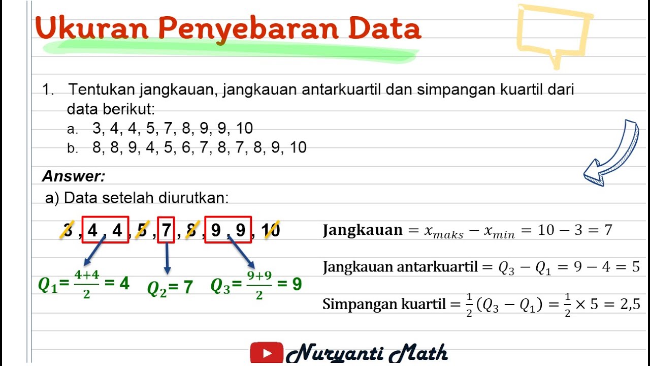
Ukuran Penyebaran Data (Jangkauan, Jangkauan Antarkuartil, Simpangan Kuartil) - STATISTIKA Kelas 8
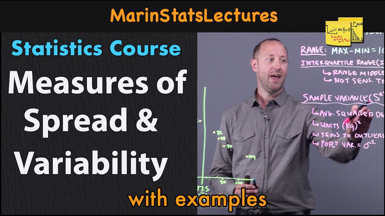
Measures of Spread & Variability: Range, Variance, SD, etc| Statistics Tutorial | MarinStatsLectures
Measures of Spread: Crash Course Statistics #4
STATISTIKA Part 2- Jangkauan, Kuartil dan Jangkauan interkuartil

Perbedaan Jangkauan, Jangkauan Interkuartil dan Kuartil pada Statistika

STATISTIKA - Cara mudah menentukan nilai Jangkauan, Jangkauan antarkuartil dan Simpangan kuartil
5.0 / 5 (0 votes)
