What is backpropagation really doing? | Chapter 3, Deep learning
Summary
TLDRThis script delves into backpropagation, the foundational algorithm for neural network learning. It offers an intuitive explanation without formulas, followed by a deeper dive into the calculus for those interested. The video covers the process of adjusting weights and biases to minimize cost functions, using the example of recognizing handwritten digits. It also touches on the practical aspects of training with large datasets, like MNIST, and the use of mini-batches for efficient stochastic gradient descent.
Takeaways
- π§ Backpropagation is the algorithm that enables neural networks to learn by calculating the gradient of the cost function with respect to the weights and biases.
- π The cost function measures the error of the network's predictions against the actual target values, and minimizing this function is the goal of learning.
- π An intuitive understanding of backpropagation involves recognizing how each training example influences the adjustments of weights and biases to decrease the cost.
- π€ The script emphasizes the importance of understanding the role of each component in the backpropagation process, despite the complexity of the notation and calculations.
- π’ The magnitude of the gradient components indicates the sensitivity of the cost function to changes in the corresponding weights and biases.
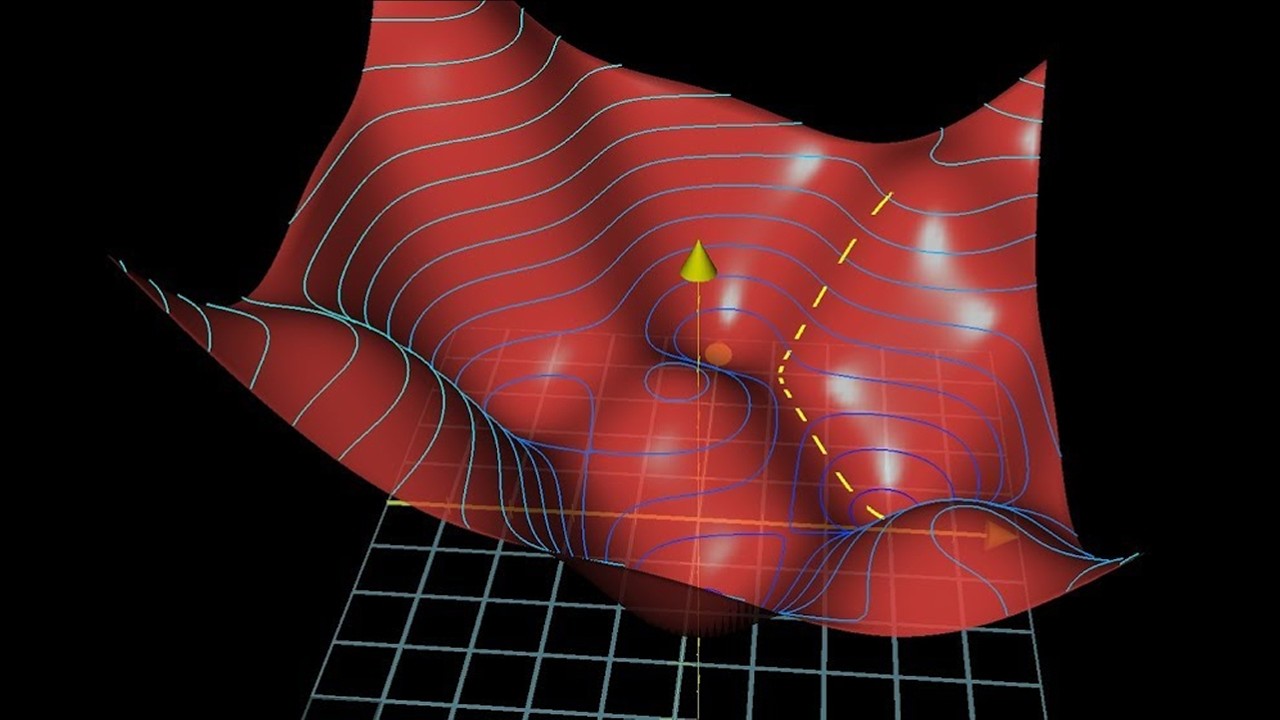
- π The negative gradient points in the direction that will most efficiently reduce the cost, guiding the adjustments made during gradient descent.
- π The process of backpropagation involves moving backwards through the network, calculating the desired changes in activations and weights from the output layer to the input layer.
- π The concept of Hebbian theory is mentioned as a loose analogy to how weights are adjusted in neural networks, with stronger connections forming between co-active neurons.
- π‘ The adjustments to weights and biases are proportional to the influence they have on the cost function, with larger adjustments made to more influential weights.
- π The script suggests that a deep understanding of backpropagation requires both an intuitive grasp of the process and a mathematical understanding of the underlying calculus.
- π» Practical implementation of backpropagation often uses mini-batches of training data for computational efficiency, a technique known as stochastic gradient descent.
Q & A
What is the core algorithm behind how neural networks learn?
-The core algorithm behind how neural networks learn is backpropagation.
What is the purpose of backpropagation in neural networks?
-The purpose of backpropagation is to compute the gradient of the cost function with respect to the weights and biases, which indicates how these parameters should be adjusted to minimize the cost and improve the network's performance.
How is the cost function defined for a single training example in the context of neural networks?
-The cost for a single training example is defined as the sum of the squares of the differences between the network's output and the desired output, for each component.
What is gradient descent and how does it relate to learning in neural networks?
-Gradient descent is an optimization algorithm used to minimize a cost function by iteratively moving in the direction of the negative gradient. In neural networks, learning involves finding the weights and biases that minimize the cost function using gradient descent.
How does the magnitude of the gradient vector components relate to the sensitivity of the cost function to changes in weights and biases?
-The magnitude of each component in the gradient vector indicates the sensitivity of the cost function to changes in the corresponding weight or bias. A larger magnitude means the cost function is more sensitive to changes in that particular weight or bias.
What is the role of the activation function in determining the output of a neuron in a neural network?
-The activation function, such as sigmoid or ReLU, is used to transform the weighted sum of inputs to a neuron, along with a bias, into the neuron's output. It introduces non-linearity into the network, allowing it to learn complex patterns.
What is the Hebbian theory in neuroscience, and how is it related to the learning process in neural networks?
-The Hebbian theory in neuroscience suggests that neurons that fire together wire together, meaning that connections between co-active neurons strengthen. This concept loosely relates to the learning process in neural networks, where weights between active neurons are increased during training.
Why is it necessary to adjust the weights and biases in proportion to their influence on the cost function?
-Adjusting the weights and biases in proportion to their influence on the cost function ensures that the most significant changes are made to the parameters that have the greatest impact on reducing the cost, leading to more efficient learning.
What is the concept of 'propagating backwards' in the context of backpropagation?
-The concept of 'propagating backwards' refers to the process of moving through the network from the output layer to the input layer, calculating the desired changes in weights and biases based on the error at each layer, which is then used to update the parameters.
What is a mini-batch in the context of stochastic gradient descent, and why is it used?
-A mini-batch is a subset of the training data used to compute a step in stochastic gradient descent. It is used to approximate the gradient of the cost function and to provide computational efficiency by not needing to process the entire dataset for each update.
What is the significance of having a large amount of labeled training data in machine learning?
-Having a large amount of labeled training data is crucial for machine learning because it allows the model to learn from a diverse set of examples, improving its ability to generalize and perform well on unseen data.
Outlines
π§ Understanding Backpropagation and Neural Networks
This paragraph introduces the concept of backpropagation, which is the fundamental learning algorithm for neural networks. It emphasizes the importance of understanding the neural network structure, the process of feeding forward information, and the concept of gradient descent. The explanation begins with an intuitive walkthrough of the algorithm without delving into complex formulas, and it sets the stage for a deeper mathematical exploration in a subsequent video. The paragraph also explains the cost function, which is used to measure the performance of the network, and how learning involves adjusting weights and biases to minimize this cost. The negative gradient of the cost function, which indicates the direction for efficient cost reduction, is highlighted as a key component of backpropagation. The explanation aims to clarify the intuition behind the algorithm, emphasizing the sensitivity of the cost function to changes in weights and biases, and how these adjustments are proportional to the desired output.
π Deep Dive into Backpropagation Mechanics
This paragraph delves deeper into the mechanics of backpropagation, focusing on how a single training example influences the adjustment of weights and biases within a neural network. It discusses the three avenues for increasing a neuron's activation: adjusting the bias, modifying the weights, and changing the activations from the previous layer. The paragraph highlights the differential impact of weights based on the activation levels of the preceding layer, drawing a parallel to Hebbian theory in neuroscience. The concept of propagating desired changes backward through the network is introduced, where the adjustments from the output layer are cascaded back to the earlier layers. The process of averaging these adjustments over multiple training examples to approximate the negative gradient of the cost function is explained, setting the groundwork for the practical application of backpropagation in training neural networks.
π Stochastic Gradient Descent and Training Data Importance
The final paragraph discusses the practical implementation of backpropagation through stochastic gradient descent, a technique that uses mini-batches of training data to approximate the gradient of the cost function. This method is presented as a computationally efficient alternative to using the entire dataset for each gradient descent step. The paragraph emphasizes the importance of having a large amount of labeled training data, using the MNIST database of handwritten digits as an example, and touches on the common challenge of acquiring sufficient training data in machine learning. It concludes by summarizing the key points of backpropagation, its role in adjusting the weights and biases of a neural network, and the iterative process of convergence towards a local minimum of the cost function.
Mindmap
Keywords
π‘Backpropagation
π‘Neural Networks
π‘Gradient Descent
π‘Cost Function
π‘Activation
π‘Weights
π‘Biases
π‘Hebbian Theory
π‘Mini-Batches
π‘Stochastic Gradient Descent
π‘MNIST Database
Highlights
Backpropagation is the core algorithm for how neural networks learn.
An intuitive walkthrough of the algorithm without formulas is provided for better understanding.
Neural networks are explained with the classic example of recognizing handwritten digits.
The importance of understanding gradient descent for learning in neural networks is emphasized.
Learning involves finding weights and biases that minimize a cost function.
The cost function is calculated by averaging the squared differences between network output and desired output.
The negative gradient of the cost function indicates how to change weights and biases to decrease the cost efficiently.
Backpropagation computes the gradient for adjusting weights and biases.
The gradient vector's magnitude represents the sensitivity of the cost function to each weight and bias.
Notation and index chasing can be confusing in understanding backpropagation.
Each training example's effect on weight and bias adjustment is explained.
Desired changes in output activations are proportional to how far they are from target values.
Adjustments in weights and biases are influenced by the activation levels of the previous layer.
Hebbian theory is mentioned as a loose analogy to how artificial neural networks learn.
The process of propagating desired changes backward through the network is described.
Averaging desired changes from all training examples gives the negative gradient of the cost function.
Stochastic gradient descent is used for computational efficiency by using mini-batches of training data.
The necessity of a large amount of training data for machine learning algorithms is highlighted.
The MNIST database is cited as an example of a valuable resource for training data in machine learning.
Transcripts
Here, we tackle backpropagation, the core algorithm behind how neural networks learn.
After a quick recap for where we are, the first thing I'll do is an intuitive walkthrough
for what the algorithm is actually doing, without any reference to the formulas.
Then, for those of you who do want to dive into the math,
the next video goes into the calculus underlying all this.
If you watched the last two videos, or if you're just jumping in with the appropriate
background, you know what a neural network is, and how it feeds forward information.
Here, we're doing the classic example of recognizing handwritten digits whose pixel
values get fed into the first layer of the network with 784 neurons,
and I've been showing a network with two hidden layers having just 16 neurons each,
and an output layer of 10 neurons, indicating which digit the network is choosing
as its answer.
I'm also expecting you to understand gradient descent,
as described in the last video, and how what we mean by learning is
that we want to find which weights and biases minimize a certain cost function.
As a quick reminder, for the cost of a single training example,
you take the output the network gives, along with the output you wanted it to give,
and add up the squares of the differences between each component.
Doing this for all of your tens of thousands of training examples and
averaging the results, this gives you the total cost of the network.
And as if that's not enough to think about, as described in the last video,
the thing that we're looking for is the negative gradient of this cost function,
which tells you how you need to change all of the weights and biases,
all of these connections, so as to most efficiently decrease the cost.
Backpropagation, the topic of this video, is an
algorithm for computing that crazy complicated gradient.
And the one idea from the last video that I really want you to hold
firmly in your mind right now is that because thinking of the gradient
vector as a direction in 13,000 dimensions is, to put it lightly,
beyond the scope of our imaginations, there's another way you can think about it.
The magnitude of each component here is telling you how
sensitive the cost function is to each weight and bias.
For example, let's say you go through the process I'm about to describe,
and you compute the negative gradient, and the component associated with the weight on
this edge here comes out to be 3.2, while the component associated with this edge here
comes out as 0.1.
The way you would interpret that is that the cost of the function is 32 times
more sensitive to changes in that first weight,
so if you were to wiggle that value just a little bit,
it's going to cause some change to the cost, and that change is 32 times greater
than what the same wiggle to that second weight would give.
Personally, when I was first learning about backpropagation,
I think the most confusing aspect was just the notation and the index chasing of it all.
But once you unwrap what each part of this algorithm is really doing,
each individual effect it's having is actually pretty intuitive,
it's just that there's a lot of little adjustments getting layered on top of each other.
So I'm going to start things off here with a complete disregard for the notation,
and just step through the effects each training example has on the weights and biases.
Because the cost function involves averaging a certain cost per example over
all the tens of thousands of training examples,
the way we adjust the weights and biases for a single gradient descent step also
depends on every single example.
Or rather, in principle it should, but for computational efficiency we'll do a little
trick later to keep you from needing to hit every single example for every step.
In other cases, right now, all we're going to do is focus
our attention on one single example, this image of a 2.
What effect should this one training example have
on how the weights and biases get adjusted?
Let's say we're at a point where the network is not well trained yet,
so the activations in the output are going to look pretty random,
maybe something like 0.5, 0.8, 0.2, on and on.
We can't directly change those activations, we
only have influence on the weights and biases.
But it's helpful to keep track of which adjustments
we wish should take place to that output layer.
And since we want it to classify the image as a 2,
we want that third value to get nudged up while all the others get nudged down.
Moreover, the sizes of these nudges should be proportional
to how far away each current value is from its target value.
For example, the increase to that number 2 neuron's activation
is in a sense more important than the decrease to the number 8 neuron,
which is already pretty close to where it should be.
So zooming in further, let's focus just on this one neuron,
the one whose activation we wish to increase.
Remember, that activation is defined as a certain weighted sum of all
the activations in the previous layer, plus a bias,
which is all then plugged into something like the sigmoid squishification function,
or a ReLU.
So there are three different avenues that can
team up together to help increase that activation.
You can increase the bias, you can increase the weights,
and you can change the activations from the previous layer.
Focusing on how the weights should be adjusted,
notice how the weights actually have differing levels of influence.
The connections with the brightest neurons from the preceding layer have the
biggest effect since those weights are multiplied by larger activation values.
So if you were to increase one of those weights,
it actually has a stronger influence on the ultimate cost function than increasing
the weights of connections with dimmer neurons,
at least as far as this one training example is concerned.
Remember, when we talk about gradient descent,
we don't just care about whether each component should get nudged up or down,
we care about which ones give you the most bang for your buck.
This, by the way, is at least somewhat reminiscent of a theory in
neuroscience for how biological networks of neurons learn, Hebbian theory,
often summed up in the phrase, neurons that fire together wire together.
Here, the biggest increases to weights, the biggest strengthening of connections,
happens between neurons which are the most active,
and the ones which we wish to become more active.
In a sense, the neurons that are firing while seeing a 2 get more
strongly linked to those are the ones firing when thinking about a 2.
To be clear, I'm not in a position to make statements one way or another about
whether artificial networks of neurons behave anything like biological brains,
and this fires together wire together idea comes with a couple meaningful asterisks,
but taken as a very loose analogy, I find it interesting to note.
Anyway, the third way we can help increase this neuron's
activation is by changing all the activations in the previous layer.
Namely, if everything connected to that digit 2 neuron with a positive
weight got brighter, and if everything connected with a negative weight got dimmer,
then that digit 2 neuron would become more active.
And similar to the weight changes, you're going to get the most bang for your buck
by seeking changes that are proportional to the size of the corresponding weights.
Now of course, we cannot directly influence those activations,
we only have control over the weights and biases.
But just as with the last layer, it's helpful
to keep a note of what those desired changes are.
But keep in mind, zooming out one step here, this
is only what that digit 2 output neuron wants.
Remember, we also want all the other neurons in the last layer to become less active,
and each of those other output neurons has its own thoughts about
what should happen to that second to last layer.
So, the desire of this digit 2 neuron is added together with the
desires of all the other output neurons for what should happen to this
second to last layer, again in proportion to the corresponding weights,
and in proportion to how much each of those neurons needs to change.
This right here is where the idea of propagating backwards comes in.
By adding together all these desired effects, you basically get a
list of nudges that you want to happen to this second to last layer.
And once you have those, you can recursively apply the same process to the
relevant weights and biases that determine those values,
repeating the same process I just walked through and moving backwards through the network.
And zooming out a bit further, remember that this is all just how a single
training example wishes to nudge each one of those weights and biases.
If we only listened to what that 2 wanted, the network would
ultimately be incentivized just to classify all images as a 2.
So what you do is go through this same backprop routine for every other training example,
recording how each of them would like to change the weights and biases,
and average together those desired changes.
This collection here of the averaged nudges to each weight and bias is,
loosely speaking, the negative gradient of the cost function referenced
in the last video, or at least something proportional to it.
I say loosely speaking only because I have yet to get quantitatively precise
about those nudges, but if you understood every change I just referenced,
why some are proportionally bigger than others,
and how they all need to be added together, you understand the mechanics for
what backpropagation is actually doing.
By the way, in practice, it takes computers an extremely long time to
add up the influence of every training example every gradient descent step.
So here's what's commonly done instead.
You randomly shuffle your training data and then divide it into a whole
bunch of mini-batches, let's say each one having 100 training examples.
Then you compute a step according to the mini-batch.
It's not going to be the actual gradient of the cost function,
which depends on all of the training data, not this tiny subset,
so it's not the most efficient step downhill, but each mini-batch does give
you a pretty good approximation, and more importantly,
it gives you a significant computational speedup.
If you were to plot the trajectory of your network under the relevant cost surface,
it would be a little more like a drunk man stumbling aimlessly down a hill but taking
quick steps, rather than a carefully calculating man determining the exact downhill
direction of each step before taking a very slow and careful step in that direction.
This technique is referred to as stochastic gradient descent.
There's a lot going on here, so let's just sum it up for ourselves, shall we?
Backpropagation is the algorithm for determining how a single training
example would like to nudge the weights and biases,
not just in terms of whether they should go up or down,
but in terms of what relative proportions to those changes cause the
most rapid decrease to the cost.
A true gradient descent step would involve doing this for all your tens of
thousands of training examples and averaging the desired changes you get.
But that's computationally slow, so instead you randomly subdivide the
data into mini-batches and compute each step with respect to a mini-batch.
Repeatedly going through all of the mini-batches and making these adjustments,
you will converge towards a local minimum of the cost function,
which is to say your network will end up doing a really good job on the training examples.
So with all of that said, every line of code that would go into implementing backprop
actually corresponds with something you have now seen, at least in informal terms.
But sometimes knowing what the math does is only half the battle,
and just representing the damn thing is where it gets all muddled and confusing.
So for those of you who do want to go deeper, the next video goes through the same
ideas that were just presented here, but in terms of the underlying calculus,
which should hopefully make it a little more familiar as you see the topic in other
resources.
Before that, one thing worth emphasizing is that for this algorithm to work,
and this goes for all sorts of machine learning beyond just neural networks,
you need a lot of training data.
In our case, one thing that makes handwritten digits such a nice example is that
there exists the MNIST database, with so many examples that have been labeled by humans.
So a common challenge that those of you working in machine learning will be familiar with
is just getting the labeled training data you actually need,
whether that's having people label tens of thousands of images,
or whatever other data type you might be dealing with.
Browse More Related Video
Gradient descent, how neural networks learn | Chapter 2, Deep learning
Neural Networks Explained in 5 minutes
Backpropagation calculus | Chapter 4, Deep learning
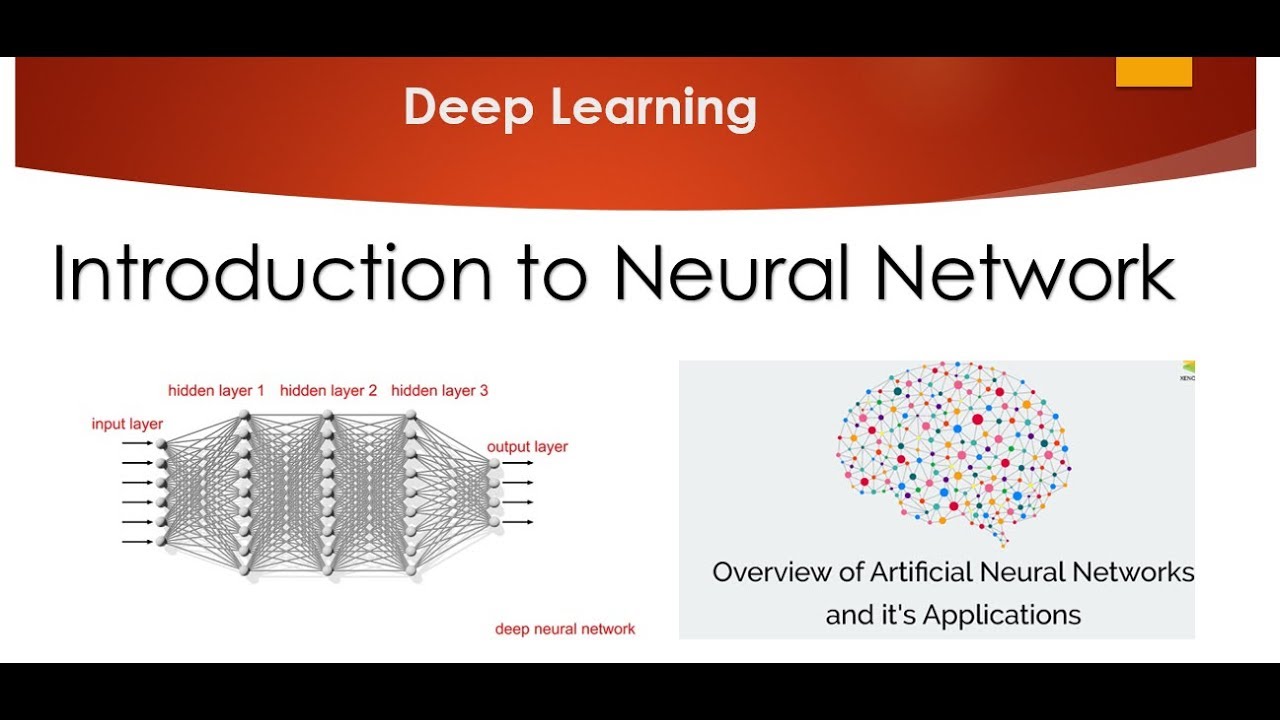
Gradient Descent, Step-by-Step
LLM Chronicles #3.1: Loss Function and Gradient Descent (ReUpload)
Neural Networks Pt. 2: Backpropagation Main Ideas
5.0 / 5 (0 votes)