EPANET Tutorial 02.03 - Project Setup | Hydraulic Modeling
Summary
TLDRIn this tutorial, Mark Wilson, founder of A Q Model, guides viewers through setting up a project in EPANET version 2.3, focusing on project defaults and ID labels. He explains how to use auto-increment for unique identifiers, set property defaults for nodes and pipes, and choose flow units between SI and English standards. Wilson also touches on head loss formulas, accuracy settings, and default patterns, providing foundational knowledge for hydraulic modeling enthusiasts.
Takeaways
- 📚 The video is a tutorial by Mark Wilson, founder of a Q model, focusing on EPANET version 2.
- 🔍 It follows the EPANET User's Manual, section by section, with advanced topics in a separate playlist.
- 🏗️ The tutorial covers project setup, specifically section 2.3 of the manual.
- 🆔 Discusses 'Project Defaults' and the importance of setting ID labels for auto-generated IDs.
- 📏 Explains how to set property defaults like node elevation, tank diameter, height, and pipe length.
- 🔗 Highlights the use of 'auto lengths' for calculating pipe length based on a properly set background map.
- 🌀 Details the significance of choosing the right flow units, which affects all units in the model including length and diameter.
- 🔢 Points out that the core unit in EPANET is cubic feet per second (CFS) and feet, with other settings converted in the background.
- ⚙️ Mentions the selection of head loss formula (Hazen-Williams, Darcy-Weisbach, or Manning) and the importance of accuracy settings.
- 🚫 Advises against setting the accuracy too high to avoid node continuity problems.
- 🌧️ Notes the default pattern setting in EPANET, which can affect how unassigned demands are handled.
- 🖼️ Discusses view dimensions and options for setting up the map area and model visualization.
Q & A
Who is the speaker in the video?
-The speaker is Mark Wilson, the founder of a Q model.
What is the main topic of the video?
-The main topic is the project setup in EPANET version two, as outlined in section 2.3 of the EPANET user's manual.
What is the purpose of the 'ID labels' tab in the project defaults?
-The 'ID labels' tab is used to prepend a piece of text to each automatically generated ID, helping to identify and organize model components.
Why is it important to set the flow units at the beginning of the project?
-Setting the flow units at the beginning is crucial as it determines whether the model uses SI units or English standard units, affecting all related measurements such as length and diameter.
What is the significance of the 'auto increment' in the ID labels tab?
-The 'auto increment' ensures that each new ID is unique, incrementing by a set number after each entry, which is essential for distinguishing different model components.
What is the default flow unit in EPANET, and why is it important?
-The default flow unit in EPANET is cubic feet per second (CFS). It's important because it serves as the core unit for all flow-related calculations in the model.
What are the three options for head loss formula in EPANET?
-The three options for head loss formula are Hazen-Williams, Darcy-Weisbach, and Jessen-Manning.
Why might a user choose a non-standard value for pipe roughness, such as 19.99?
-A non-standard value like 19.99 can serve as a flag to indicate that no engineering judgment was used in determining the roughness, allowing for adjustments during the calibration process.
What is the role of the 'default pattern' setting in EPANET?
-The 'default pattern' setting ensures that any demand not specifying a pattern other than one will adopt that pattern, which can be crucial for uniformity in demand distribution.
What does the 'global demand multiplier' setting do in the model?
-The 'global demand multiplier' allows for quick adjustments to peak demands, such as during the max day or max hour, providing a simple way to scale demand across the model.
Why is the 'view options' section important for the model setup?
-The 'view options' section is important for setting up the visual aspects of the model, including symbology, flow arrows, and background color, which aid in the model's interpretation and analysis.
Outlines

This section is available to paid users only. Please upgrade to access this part.
Upgrade NowMindmap

This section is available to paid users only. Please upgrade to access this part.
Upgrade NowKeywords

This section is available to paid users only. Please upgrade to access this part.
Upgrade NowHighlights

This section is available to paid users only. Please upgrade to access this part.
Upgrade NowTranscripts

This section is available to paid users only. Please upgrade to access this part.
Upgrade NowBrowse More Related Video
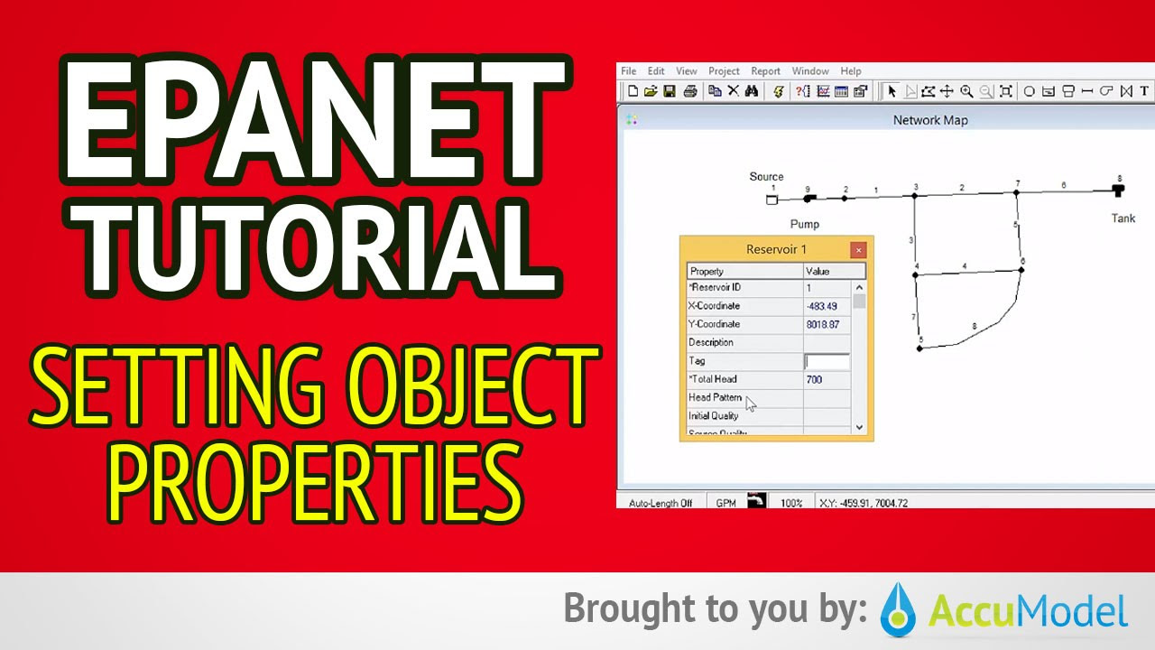
EPANET Tutorial 02.05 - Setting Object Properties | Hydraulic Modeling
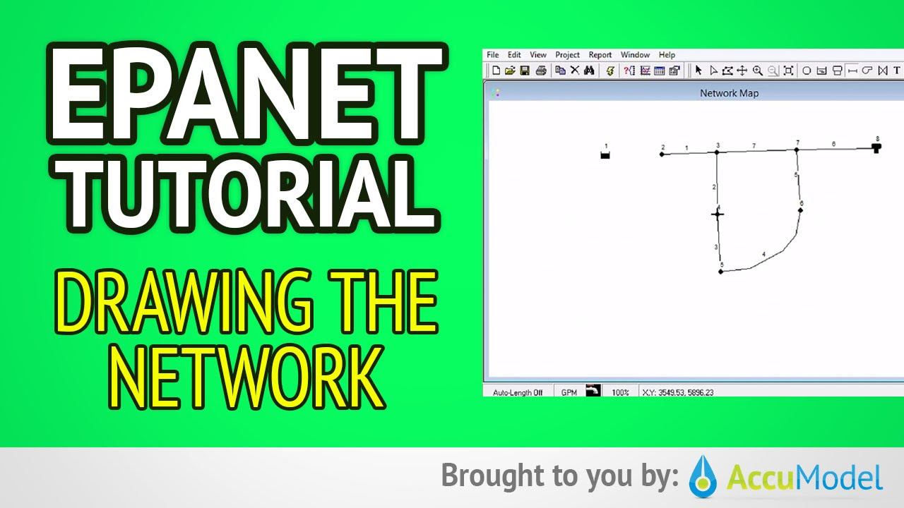
EPANET Tutorial 02.04 - Drawing The Network | Hydraulic Modeling
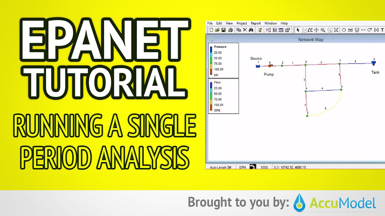
EPANET Tutorial 02.07 - Running a Single Period Analysis | Hydraulic Modeling

EPANET Tutorial 02.06 - Saving and Opening Projects | Hydraulic Modeling

Django Testing Tutorial with Pytest #1 - Setup (2018)

EPANET Tutorial 01 - Overview of EPANET | Hydraulic Modeling
5.0 / 5 (0 votes)