Complex Integration In Plain English
Summary
TLDRThis video introduces complex integration, explaining how to visualize complex functions using vector fields. It shows how the integral of a complex function along a contour can be understood as the work done by the function's vector field pushing a particle along the contour. An example is provided evaluating the integral of 1/z^2 around the unit circle, using intuition about the vector field's symmetry to predict the result will be 0 before confirming with calculation. The video concludes by previewing upcoming explanations of Cauchy's integral formula and the residue theorem in the next videos of this complex integration series.
Takeaways
- 😊 Vector fields can be used to visualize complex functions by mapping the function's real part to the x-component and imaginary part to the y-component of a vector at each point.
- 📏 To define a complex integral, we need to specify the integration contour/path in the complex plane, unlike in real integration.
- ⛺ Closed integration contours are denoted with a circle in the integral symbol.
- 🚏 The complex integral can be interpreted as the work done by the function's vector field along the contour.
- 🌀 The integral's real part gives the work and imaginary part gives the flux of the vector field along the contour.
- 🎯 Solved an example problem of evaluating the integral of 1/z^2 along the unit circle using vector field intuition.
- 👀 Discussed and visualized vector fields of functions and their conjugates, known as POA vector fields.
- 🔬 Parameterized the integration contour and derived a general formula for complex line integrals.
- 📝 Showed how Euler's formula can provide an alternative interpretation of the complex integral.
- ⏩ Upcoming topics include Cauchy's formulas and residue theorem for complex integrals.
Q & A
How can complex functions be visualized using vector fields?
-Every point in space is assigned a vector whose x component is the real part and y component is the imaginary part of the function's output. This creates a vector field that can provide intuition about the function's behavior.
What are the limits of integration in a complex integral?
-Complex numbers can't be used as limits of integration since there are infinitely many paths between two complex points. Instead the path (contour) must be specified.
What does the complex integral represent intuitively?
-It can be seen as the work done by the function's vector field to push a particle along the contour. The real part is the work, and imaginary part is the flux.
What is a polar vector field and why is it important?
-A polar vector field represents the conjugate of the original function. These fields play an important role in evaluating complex integrals using the ideas of work and flux.
How can Cauchy's integral formula be used to evaluate complex integrals?
-Cauchy's formula allows complex integrals to be converted into integrals over the boundary contours. This allows powerful results like the residue theorem to be applied.
What is the insight behind evaluating the example integral?
-The symmetry of the vector field about the real line results in the work and flux along the unit circle contour canceling out to zero.
What topics will be covered in the next videos?
-The next videos will cover Cauchy's integral formula, Cauchy's theorem, and the residue theorem which are powerful tools for evaluating complex integrals.
How can complex functions be represented geometrically?
-Complex functions map the complex plane to itself, so they can be visualized as transforming or morphing the complex plane through stretching, rotation, translation etc.
What challenges arise in visualizing functions of complex variables?
-Complex functions have a 4-dimensional input and output space which is difficult to visualize. Methods like vector fields are needed to build intuition.
What are some applications of complex integration?
-Applications include solving differential equations, evaluation of real integrals, summing series, and problems in physics and engineering involving fields and fluid flow.
Outlines

This section is available to paid users only. Please upgrade to access this part.
Upgrade NowMindmap

This section is available to paid users only. Please upgrade to access this part.
Upgrade NowKeywords

This section is available to paid users only. Please upgrade to access this part.
Upgrade NowHighlights

This section is available to paid users only. Please upgrade to access this part.
Upgrade NowTranscripts

This section is available to paid users only. Please upgrade to access this part.
Upgrade NowBrowse More Related Video
[NEW VERSION!]GAYA COULOMB | Listrik Statis - Fisika Kelas 12

Seminário "Introdução à Modelagem Computacional" - Acadêmico Murilo Saraiva

Introduction to Complex Functions

Grafik dan Nilai Mutlak Bilangan Kompleks
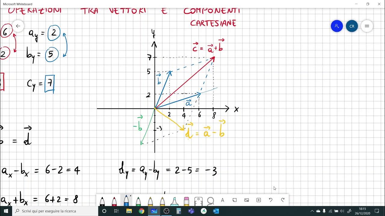
Operazioni tra vettori in componenti cartesiane

12th Physics | Chapter No 1 | Rotational Dynamics | Lecture 1 | JR Tutorials |
5.0 / 5 (0 votes)